Unit - 2

Speech Signal Processing

Q1) Define pitch period estimation?

Ans: Pitch period estimation

The fundamental frequency, or pitch, of voiced speech is one of the most important parameters in speech processing, synthesis, and coding applications. Pitch pitch is directly related to the speaker and defines a person's distinct personality. The airflow from the lungs is occasionally blocked by movements of the vocal cords, resulting in voicing. The fundamental duration, or pitch period, is the interval between successive vocal cord openings.

The theoretical pitch frequency range for men is typically between 50 and 250 Hz, while the range for women is usually between 120 and 500 Hz. A male's period ranges from 4 to 20 milliseconds, whereas a female's period ranges from 2 to 8 milliseconds.

At each frame, the pitch time must be calculated. It is possible to determine the time in which the signal repeats itself by comparing a frame to previous tests, resulting in an estimation of the real pitch period. It's worth noting that the estimation process only works for voiced frames. Because of their random existence, unvoiced frames produce meaningless effects.

Due to the lack of perfect periodicity, interference with vocal tract formants, ambiguity of the starting instance of a voiced part, and other real-world elements such as noise and echo, developing a pitch period estimation algorithm is a difficult task. Pitch period estimation is applied in practice as a compromise between computational complexity and efficiency. Just a few methods for estimating pitch time have been suggested, and only a few are included.

Q2) Define all poles and all zero filters?

Ans: Filters that have a machine feature

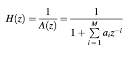
Or

are of special significance to speech coding. Since only poles are present in the equation, an all-pole filter is defined, while the system function of an all-zero filter is given. H(z) and A(z) are the inverses of each other, as we can see. The order of the filter is M, and the coefficients of the filter are ai. Both linear-prediction-based speech coders have these filters. The prediction order is also known as M, and the linear prediction coefficients are known as ai.

Direct Form Realization

With x[n] being the input to the filter and y[n] the output, the time-domain difference equation corresponding to above equation is

And for 2nd equation,

The signal flow graphs of the above difference equations are shown in Figure. Direct type filters are those that are applied in this way. Since the scaled and delayed versions of the output samples are applied back to the input samples, the impulse response of an all-pole filter has an infinite number of samples with nontrivial values. An infinite-impulse-response (IIIR) filter is what this is called. The impulse response of an all-zero filter, on the other hand, only has M + 1 nontrivial samples (the rest are zeros) and is referred to as a finite-impulse-response (FIR) filter.

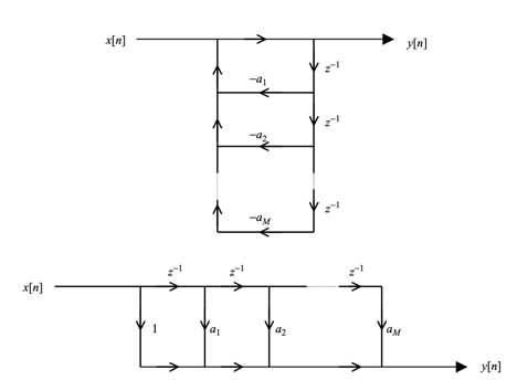
Fig 1: Signal flow graph for direct form implementation of an all-pole filter (top) and all-zero filter (bottom).

Lattice Realization

Figure depicts a lattice structure as an alternate realization for the filters.

The reflection coefficients are defined by the parameters k1,..., kM. The reflection coefficients can be found using the computational loop below, which starts with the direct form coefficients (a1,..., aM).

For l = M, M - 1, ... , 1:

kl = -al(l) ;

where ai = ai (M). The above relationships are directly obtained by deriving the lattice form's input–output difference equation and comparing it to the direct form's. The set of equations for the all-pole filter is as follows:

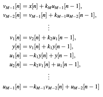
are solved in order to obtain the output series y[n]. The all-zero filter, on the other hand,

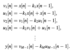
Q3) What do you mean by convolution?

Ans: We have the linear time-invariant (LTI) system with impulse response h[n], where the system's input is x[n] and output is y[n].

One of the fundamental relationships in signal processing is the convolution number between x[n] and h[n]. The convolution number, with a focus on the all-pole filter, is used to calculate the output sequence frame by frame.

Impulse Response of an All-Pole Filter

When the input is a single impulse, the time domain difference equation x[n]=d[n] is a simple way to find the impulse response series. That is right.

On a sample-by-sample basis, we've found

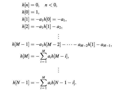
As a result, the filter coefficients decide the impulse response series.

Recursive Convolution

We define the following L sequences given the sequence x[n], n = 0,..., S(L - 1) + N - 1, with S, L, and N positive integers:

x(0)[n] =  x[n + (L -1)S];

x(1)[n] = x[n + (L -2)S];

.

.

.

 x(L-1)[n] = x[n]:

For n = 0 to N - 1, in general, we write

x(l)[n] = x[n + (L - l - 1)S;  l = 0; 1; ... ; L - 1;  n = 0; 1; ... ; n - 1

The relationship between x[n] and x(l)[n] is depicted in Figure. Keep in mind the

x(l+1)[n] = x(l)[n -S];  S  ≤ n ≤ N - 1:

To put it another way, x(l)[n] is obtained by collecting N samples from the sequence x[n] at various points. It is desirable to find a device with an impulse response of h[n].

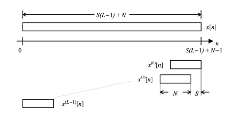
Fig 2: Obtaining the input sequences in recursive convolution

the zero-state responses that correspond to the x(l)[n] input sequences In matrix form, let's call these responses y(l)[n]:

y(l) = H. x(l)

The above equation indicates that each input sequence be subjected to an independent convolution operation in order to compute the device responses. However, since the input sequences share similar samples, the total computation can be reduced. Find the following to gain a better understanding of the situation:

Then,

Conclude that,

If the lth response is inaccessible, only the first S samples of the (l + 1)st response must be computed using the standard convolution method. A simpler, less complicated operation can be used to find the last (N - S) samples. The equation is known as recursive convolution since the convolution of one series can be found by recursively finding the convolution of the previous answer.

CELP-style speech coders often employ recursive convolution. The zero-state responses must be extracted from a codebook with overlapping code vectors.

Q4) What is power spectral density?

Ans: The power spectral density function aids in calculating the total power found in each of a signal's spectral components. Consider a sine wave with a fixed frequency; in this case, the PSD plot would only have one spectral component present at that frequency.

Simply put, the power spectrum of any time domain signal x(t) aids in the determination of the variance distribution of data x(t) over the frequency domain in the form of spectral components from which the actual signal can be decomposed. In this step, power spectral densities are calculated on the signal obtained after applying various windows.

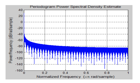
Fig 3:  Power Spectral Density of Hamming Window

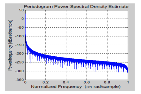
Fig 4: Power Spectral Density of Hanning Window

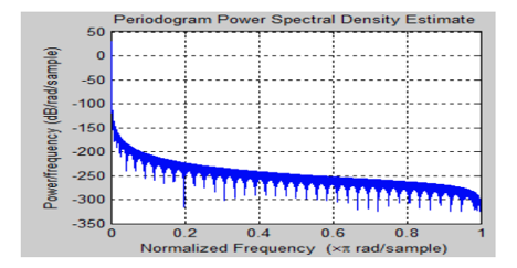
Fig 5: Power Spectral Density of Blackman Window

Above Figure shows the power spectral density plot for a given audio signal, as well as the results of Hamming, Hanning, and Blackman windows.

When a signal's energy is concentrated around a finite time interval, particularly if its total energy is finite, the energy spectral density can be computed. The power spectral density (or simply power spectrum) is a term that refers to signals that occur over time or over a time span that is broad enough (especially in relation to the length of a measurement) to be considered infinite. Since the cumulative energy of such a signal over all time will be infinite, the power spectral density (PSD) refers to the spectral energy distribution that would be found per unit time.

Q5) What do you understand by periodogram?

Ans: The periodogram is based on the power spectral density concept (PSD). Let xw(n) = ⍵(n)x(n) denote a windowed segment of samples from a random process x(n), where ⍵ (traditionally the rectangular window) contains M nonzero samples. The periodogram is then calculated by dividing the squared-magnitude DTFT of xw by M.

The predicted value of the periodogram equals the true power spectral density of the noise phase x(n) as M approaches infinity. Writing is used to express this.

where  Sx(⍵) is the power spectral density (PSD) of x and Sx(⍵) is the power spectral density (PSD) of  x. We have a sample PSD defined in terms of the sample PSD defined.

That is, the smoothed sample PSD equals the periodogram. The autocorrelation function corresponding to the periodogram is Bartlett windowed in the time domain. In practice, we compute a sampled periodogram Sx(⍵k), ⍵k = 2π/N, with the duration N ≥ M FFT replacing the DTFT. The computation of the periodogram is essentially one of the phases.

The issue with the periodogram of noise signals is that it is, for the most part, random. That is, when the Fourier transform divides the noise into bands, it is not averaged in any way that decreases randomness, and each band generates a nearly independent random value.

Q6) What do you mean by the Autoregressive model?

Ans: Any hypothesis that can be used to clarify or define the secret laws that are supposed to control or constrain the generation of some interesting data is referred to as a model. The output of an all-pole linear filter powered by white noise is a popular method for modeling random signals.

Random signals with desired spectral characteristics can be generated by selecting a filter with an acceptable denominator polynomial, since the power spectrum of the filter output is given by the constant noise spectrum multiplied by the squared magnitude of the filter.

If the difference equation is satisfied, the sequence values x[n]; x[n - l];...; x[n - M] reflect the realization of an autoregressive (AR) phase of order M.

x[n] + a1x[n - 1] + ………+ aMx[n - M] =  v[n];

The AR parameters are constants a1; a2;...; aM, and v[n] represents a white noise process; the above equation can be written as

X[n] = -a1x[n - 1] - a2x[n - 2]- ………-aMx[n - M] + v[n]

As a result, the process's current value, x[n], is equal to a linear combination of the process's past values, x[n - 1];...; x[n -M], plus an error term v[n]. x[n] is said to be regressed on x[n - 1]; x[n - 2];...; x[n - M]; in particular, x[n] is regressed on previous values of itself, hence the term "autoregressive."

System Function of the AR Process Analyzer

Using the z-transform to manipulate yields is a great way to start.

 where HA(z) denotes the AR analyzer's machine function, which is a filter that takes x[n] as input and outputs v[n]. In the equation above, the parameter a0 equals one. As a result, the AR analyzer converts an AR phase into white noise at its output. The AR analyzer's direct form realization [Oppenheim and Schafer, 1989] is shown in Figure. It's worth noting that the AR process analyzer is an all-zero filter, so it's FIR in design.

System Function of the AR Process Synthesizer

We can use the device function given by the white noise v[n] as input.

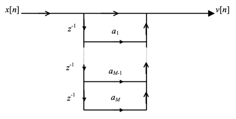
Fig 6: Direct form realization of the AR process analyzer filter

to x[n] synthesize the AR mechanism Figure depicts the realization of a direct form. The AR process synthesizer is an all-pole filter with an infinite impulse response range (IIR). The synthesizer accepts white noise as an input and outputs an AR signal. We can see that the analyzer's system function is the opposite of the synthesizer's system function; we can also write

where p1; p2; ... ; pM are poles of HS(z) and are roots of the characteristic equation

 1 + a1z-1 + a2z-2 +..........+ aMz-M = 0:

As a result, an AR phase is generated by using an all-pole filter to filter white noise.

Q7) What do you mean by Autocorrelation estimation?

Ans: Since speech is non-stationary, autocorrelation values must be estimated and updated for each short period of time; their values must be recalculated in each signal frame. Non-recursive and recursive procedures are the two basic types of procedures. The two types of estimation methods are similar to the two types of optical filters: FIR and IIR. Non-recursive methods use a finite-length window for extraction, whereas recursive methods use an infinite-length window. The program determines whether or not one of these methods is used.

* Defines the autocorrelation function of a real discrete-time signal x[n] at lag l.

Various estimators have been implemented.

Non Recursive Estimation Methods

The Hamming window is one of the most commonly used non-recursive approaches, which uses a well-defined window sequence w12n to retrieve the signal frame of interest for further processing.

The Hamming causal window is described as follows:

with N denoting the size of the window (number of nonzero samples). A plot of the window series is shown in Figure. The values of the window series are often stored in memory in operation.

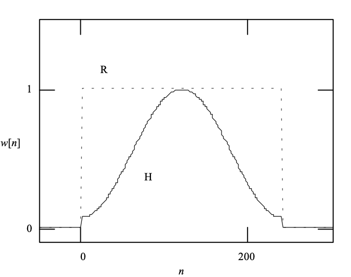
Fig 7: Plots of the rectangular and Hamming window, with a length of N = 240.

Recursive Estimation Methods

Since it is approximately the time period over which the signal remains stationary, the frame length N for most speech coding applications is on the order of 200 samples. Figure (a) shows an example of how the autocorrelation values are calculated per 200 samples using a 200-sample window.

In certain applications, it may be possible to perform the calculation in a much smaller interval than 200, such as 40. The delay associated with the buffering phase (required to collect the input samples) is significantly reduced by updating the estimates more regularly, which is highly beneficial in practice. The solution is shown in Figure (b).

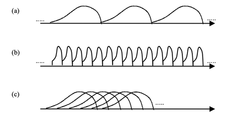
Fig 8: Non recursive autocorrelation estimation is depicted in this diagram

(a) Per 200 samples, estimation is performed using a 200-sample window.

(b) Estimation is done every 40 samples, with a 40-sample window.

(c) Estimation is done every 40 samples, with a 200-sample window. It's worth noting that the windows are overlapping.

In this case, a 40-foot window is used. A short window, on the other hand, would increase the estimates' bias, resulting in unreliable results. The situation depicted in Figure (c), where a 200-sample window is used per 40 samples, resulting in overlapping, may be used for higher precision.

Q8) What are the applications of Speech Processing?

Ans: Speech processing is the application of digital signal processing (DSP) techniques for processing and analysis of signal. Digital signal processing treats a signal as a series of numbers. Regardless of the content implied by the number, the numbers can be treated(processed) in many ways.

Applications of speech processing include:
 

Other Applications of speech processing

Q9) What do you mean by speech processing?

Ans: Speech processing

The study of speech signals and signal processing techniques is known as speech processing. Speech processing may be thought of as a special case of digital signal processing applied to speech signals since the signals are normally processed in a digital representation. Acquisition, manipulation, storage, transition, and performance of speech signals are all aspects of speech processing. Speech recognition is the input, whereas speech synthesis is the output.

Q10) What are the techniques of speech processing?

Ans: Technique of speech processing

Dynamic time warping (DTW) - is an algorithm for determining the similarity of two temporal sequences that may differ in speed. In general, DTW is a tool for finding the best fit between two sequences (e.g., time series) under certain constraints and laws. The optimal match is defined as the one that satisfies all of the restrictions and rules while also having the lowest cost, where the cost is calculated as the total of absolute differences between the values of each matched pair of indices.

Hidden Markov models - The simplest dynamic Bayesian network can be interpreted as a hidden Markov model. The algorithm's aim is to find a hidden variable x(t) from a set of observations y. (t). Given the values of the hidden variable x at all times, the conditional probability distribution of the hidden variable x(t) at time t is only dependent on the value of the hidden variable x(t 1). Similarly, the observed variable y(t) is solely determined by the value of the hidden variable x(t) (both at time t).

Artificial neural networks - An artificial neural network (ANN) is made up of artificial neurons, which are a series of linked units or nodes that loosely model the neurons in a biological brain. Each link can send a signal from one artificial neuron to another, just like synapses in a biological brain. When an artificial neuron receives a signal, it may interpret it and then send it to other artificial neurons. The signal at a link between artificial neurons is a real number in most ANN implementations, and the output of each artificial neuron is computed by some non-linear function of the sum of its inputs.

Phase-aware processing - Phase is usually supposed to be a random uniform variable and thus useless. This is due wrapping of phase: result of arctangent function is not continuous due to periodical jumps on

{\displaystyle 2\p

. After phase unwrapping , it can be expressed as:

{\displaystyle \phi (h,l)=\phi _{lin}(h,l)+\Psi (h,l)}

, where

{\displaystyle \phi _{lin}(h,l)=\omega _{0}(l'){}_{\Delta }t}

is linear phase (

{\displaystyle {}_{\Delta }t}

is temporal shift at each frame of analysis),

{\displaystyle \Psi (h,l)}

is phase contribution of the vocal tract and phase source. Obtained phase estimations can be used for noise reduction: temporal smoothing of instantaneous phase and its derivatives by time (instantaneous frequency) and frequency (group delay), smoothing of phase across frequency.  Joined amplitude and phase estimators can recover speech more accurately based on assumption of von Mises distribution of phase.