UNIT 3

1. Explain learning in brief

Machine Learning (ML) is an automated learning with little or no human intervention. It involves programming computers so that they learn from the available inputs. The main purpose of machine learning is to explore and construct algorithms that can learn from the previous data and make predictions on new input data.

The input to a learning algorithm is training data, representing experience, and the output is any expertise, which usually takes the form of another algorithm that can perform a task. The input data to a machine learning system can be numerical, textual, audio, visual, or multimedia. The corresponding output data of the system can be a floating-point number, for instance, the velocity of a rocket, an integer representing a category or a class, for example, a pigeon or a sunflower from image recognition.

In this chapter, we will learn about the training data our programs will access and how learning process is automated and how the success and performance of such machine learning algorithms is evaluated.

Concepts of Learning

Learning is the process of converting experience into expertise or knowledge.

Learning can be broadly classified into three categories, as mentioned below, based on the nature of the learning data and interaction between the learner and the environment.

• Supervised Learning
• Unsupervised Learning
• Semi-supervised Learning

Similarly, there are four categories of machine learning algorithms as shown below −

• Supervised learning algorithm
• Unsupervised learning algorithm
• Semi-supervised learning algorithm
• Reinforcement learning algorithm

However, the most commonly used ones are supervised and unsupervised learning.

2.     What is Supervised Learning?

Supervised learning is commonly used in real world applications, such as face and speech recognition, products or movie recommendations, and sales forecasting. Supervised learning can be further classified into two types - Regression and Classification.

Regression trains on and predicts a continuous-valued response, for example predicting real estate prices.

Classification attempts to find the appropriate class label, such as analyzing positive/negative sentiment, male and female persons, benign and malignant tumors, secure and unsecure loans etc.

In supervised learning, learning data comes with description, labels, targets or desired outputs and the objective is to find a general rule that maps inputs to outputs. This kind of learning data is called labeled data. The learned rule is then used to label new data with unknown outputs.

Supervised learning involves building a machine learning model that is based on labeled samples. For example, if we build a system to estimate the price of a plot of land or a house based on various features, such as size, location, and so on, we first need to create a database and label it. We need to teach the algorithm what features correspond to what prices. Based on this data, the algorithm will learn how to calculate the price of real estate using the values of the input features.

Supervised learning deals with learning a function from available training data. Here, a learning algorithm analyzes the training data and produces a derived function that can be used for mapping new examples. There are many supervised learning algorithms such as Logistic Regression, Neural networks, Support Vector Machines (SVMs), and Naive Bayes classifiers.

Common examples of supervised learning include classifying e-mails into spam and not-spam categories, labeling webpages based on their content, and voice recognition.

3.     Explain categories of learning

Unsupervised Learning

Unsupervised learning is used to detect anomalies, outliers, such as fraud or defective equipment, or to group customers with similar behaviors for a sales campaign. It is the opposite of supervised learning. There is no labeled data here.

When learning data contains only some indications without any description or labels, it is up to the coder or to the algorithm to find the structure of the underlying data, to discover hidden patterns, or to determine how to describe the data. This kind of learning data is called unlabeled data.

Suppose that we have a number of data points, and we want to classify them into several groups. We may not exactly know what the criteria of classification would be. So, an unsupervised learning algorithm tries to classify the given dataset into a certain number of groups in an optimum way.

Unsupervised learning algorithms are extremely powerful tools for analyzing data and for identifying patterns and trends. They are most commonly used for clustering similar input into logical groups. Unsupervised learning algorithms include Kmeans, Random Forests, Hierarchical clustering and so on.

Semi-supervised Learning

If some learning samples are labeled, but some other are not labeled, then it is semi-supervised learning. It makes use of a large amount of unlabeled data for training and a small amount of labeled data for testing. Semi-supervised learning is applied in cases where it is expensive to acquire a fully labeled dataset while more practical to label a small subset. For example, it often requires skilled experts to label certain remote sensing images, and lots of field experiments to locate oil at a particular location, while acquiring unlabeled data is relatively easy.

Reinforcement Learning

Here learning data gives feedback so that the system adjusts to dynamic conditions in order to achieve a certain objective. The system evaluates its performance based on the feedback responses and reacts accordingly. The best known instances include self-driving cars and chess master algorithm AlphaGo.

4.     Explain Introduction to K-Means Algorithm

K-means clustering algorithm computes the centroids and iterates until we it finds optimal centroid. It assumes that the number of clusters are already known. It is also called flat clustering algorithm. The number of clusters identified from data by algorithm is represented by ‘K’ in K-means.

In this algorithm, the data points are assigned to a cluster in such a manner that the sum of the squared distance between the data points and centroid would be minimum. It is to be understood that less variation within the clusters will lead to more similar data points within same cluster.

Working of K-Means Algorithm

We can understand the working of K-Means clustering algorithm with the help of following steps −

Step 1 − First, we need to specify the number of clusters, K, need to be generated by this algorithm.

Step 2 − Next, randomly select K data points and assign each data point to a cluster. In simple words, classify the data based on the number of data points.

Step 3 − Now it will compute the cluster centroids.

Step 4 − Next, keep iterating the following until we find optimal centroid which is the assignment of data points to the clusters that are not changing any more

• 4.1 − First, the sum of squared distance between data points and centroids would be computed.
• 4.2 − Now, we have to assign each data point to the cluster that is closer than other cluster (centroid).
• 4.3 − At last compute the centroids for the clusters by taking the average of all data points of that cluster.

K-means follows Expectation-Maximization approach to solve the problem. The Expectation-step is used for assigning the data points to the closest cluster and the Maximization-step is used for computing the centroid of each cluster.

While working with K-means algorithm we need to take care of the following things −

• While working with clustering algorithms including K-Means, it is recommended to standardize the data because such algorithms use distance-based measurement to determine the similarity between data points.
• Due to the iterative nature of K-Means and random initialization of centroids, K-Means may stick in a local optimum and may not converge to global optimum. That is why it is recommended to use different initializations of centroids.

5.     Explain Implementation in Python of K-Means Algorithm with some examples

The following two examples of implementing K-Means clustering algorithm will help us in its better understanding −

Example 1

It is a simple example to understand how k-means works. In this example, we are going to first generate 2D dataset containing 4 different blobs and after that will apply k-means algorithm to see the result.

First, we will start by importing the necessary packages −

%matplotlib inline

Import matplotlib.pyplot as plt

Import seaborn as sns; sns.set()

Import numpy as np

From sklearn.cluster import KMeans

The following code will generate the 2D, containing four blobs −

From sklearn.datasets.samples_generator import make_blobs

X, y_true = make_blobs(n_samples = 400, centers = 4, cluster_std = 0.60, random_state = 0)

Next, the following code will help us to visualize the dataset −

Plt.scatter(X[:, 0], X[:, 1], s = 20);

Plt.show()

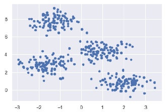
Next, make an object of KMeans along with providing number of clusters, train the model and do the prediction as follows −

Kmeans = KMeans(n_clusters = 4)

Kmeans.fit(X)

y_kmeans = kmeans.predict(X)

Now, with the help of following code we can plot and visualize the cluster’s centers picked by k-means Python estimator −

From sklearn.datasets.samples_generator import make_blobs

X, y_true = make_blobs(n_samples = 400, centers = 4, cluster_std = 0.60, random_state = 0)

Next, the following code will help us to visualize the dataset −

Plt.scatter(X[:, 0], X[:, 1], c = y_kmeans, s = 20, cmap = 'summer')

Centers = kmeans.cluster_centers_

Plt.scatter(centers[:, 0], centers[:, 1], c = 'blue', s = 100, alpha = 0.9);

Plt.show()

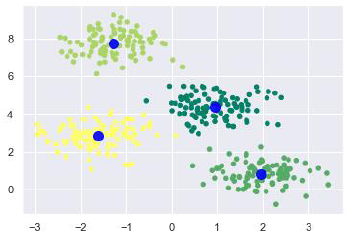
Example 2

Let us move to another example in which we are going to apply K-means clustering on simple digits dataset. K-means will try to identify similar digits without using the original label information.

First, we will start by importing the necessary packages −

%matplotlib inline

Import matplotlib.pyplot as plt

Import seaborn as sns; sns.set()

Import numpy as np

From sklearn.cluster import KMeans

Next, load the digit dataset from sklearn and make an object of it. We can also find number of rows and columns in this dataset as follows −

From sklearn.datasets import load_digits

Digits = load_digits()

Digits.data.shape

Output

(1797, 64)

The above output shows that this dataset is having 1797 samples with 64 features.

We can perform the clustering as we did in Example 1 above −

Kmeans = KMeans(n_clusters = 10, random_state = 0)

Clusters = kmeans.fit_predict(digits.data)

Kmeans.cluster_centers_.shape

Output

(10, 64)

The above output shows that K-means created 10 clusters with 64 features.

Fig, ax = plt.subplots(2, 5, figsize=(8, 3))

Centers = kmeans.cluster_centers_.reshape(10, 8, 8)

For axi, center in zip(ax.flat, centers):

Axi.set(xticks=[], yticks=[])

Axi.imshow(center, interpolation='nearest', cmap=plt.cm.binary)

Output

As output, we will get following image showing clusters centers learned by k-means.

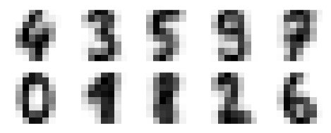
The following lines of code will match the learned cluster labels with the true labels found in them −

From scipy.stats import mode

Labels = np.zeros_like(clusters)

For i in range(10):

   mask = (clusters == i)

   labels[mask] = mode(digits.target[mask])[0]

Next, we can check the accuracy as follows −

From sklearn.metrics import accuracy_score

Accuracy_score(digits.target, labels)

Output

0.7935447968836951

The above output shows that the accuracy is around 80%.

6.     What are the Advantages and Disadvantages of K-Means clustering algorithms and write its applications?

Advantages

The following are some advantages of K-Means clustering algorithms −

• It is very easy to understand and implement.
• If we have large number of variables then, K-means would be faster than Hierarchical clustering.
• On re-computation of centroids, an instance can change the cluster.
• Tighter clusters are formed with K-means as compared to Hierarchical clustering.

Disadvantages

The following are some disadvantages of K-Means clustering algorithms −

• It is a bit difficult to predict the number of clusters i.e. the value of k.
• Output is strongly impacted by initial inputs like number of clusters (value of k)
• Order of data will have strong impact on the final output.
• It is very sensitive to rescaling. If we will rescale our data by means of normalization or standardization, then the output will completely change.
• It is not good in doing clustering job if the clusters have a complicated geometric shape.

Applications of K-Means Clustering Algorithm

The main goals of cluster analysis are −

• To get a meaningful intuition from the data we are working with.
• Cluster-then-predict where different models will be built for different subgroups.

To fulfill the above-mentioned goals, K-means clustering is performing well enough. It can be used in following applications −

• Market segmentation
• Document Clustering
• Image segmentation
• Image compression
• Customer segmentation
• Analyzing the trend on dynamic data

7.     How does the Decision Tree algorithm Work?

In a decision tree, for predicting the class of the given dataset, the algorithm starts from the root node of the tree. This algorithm compares the values of root attribute with the record (real dataset) attribute and, based on the comparison, follows the branch and jumps to the next node.

For the next node, the algorithm again compares the attribute value with the other sub-nodes and move further. It continues the process until it reaches the leaf node of the tree. The complete process can be better understood using the below algorithm:

• Step-1: Begin the tree with the root node, says S, which contains the complete dataset.
• Step-2: Find the best attribute in the dataset using Attribute Selection Measure (ASM).
• Step-3: Divide the S into subsets that contains possible values for the best attributes.
• Step-4: Generate the decision tree node, which contains the best attribute.
• Step-5: Recursively make new decision trees using the subsets of the dataset created in step -3. Continue this process until a stage is reached where you cannot further classify the nodes and called the final node as a leaf node.

Example: Suppose there is a candidate who has a job offer and wants to decide whether he should accept the offer or Not. So, to solve this problem, the decision tree starts with the root node (Salary attribute by ASM). The root node splits further into the next decision node (distance from the office) and one leaf node based on the corresponding labels. The next decision node further gets split into one decision node (Cab facility) and one leaf node. Finally, the decision node splits into two leaf nodes (Accepted offers and Declined offer). Consider the below diagram:

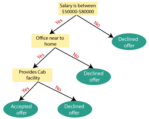
Attribute Selection Measures

While implementing a Decision tree, the main issue arises that how to select the best attribute for the root node and for sub-nodes. So, to solve such problems there is a technique which is called as Attribute selection measure or ASM. By this measurement, we can easily select the best attribute for the nodes of the tree. There are two popular techniques for ASM, which are:

• Information Gain
• Gini Index

1. Information Gain:

• Information gain is the measurement of changes in entropy after the segmentation of a dataset based on an attribute.
• It calculates how much information a feature provides us about a class.
• According to the value of information gain, we split the node and build the decision tree.
• A decision tree algorithm always tries to maximize the value of information gain, and a node/attribute having the highest information gain is split first. It can be calculated using the below formula:

1. Information Gain= Entropy(S)- [(Weighted Avg) *Entropy(each feature)  

Entropy: Entropy is a metric to measure the impurity in a given attribute. It specifies randomness in data. Entropy can be calculated as:

Entropy(s)= -P(yes)log2 P(yes)- P(no) log2 P(no)

Where,

• S= Total number of samples
• P(yes)= probability of yes
• P(no)= probability of no

2. Gini Index:

• Gini index is a measure of impurity or purity used while creating a decision tree in the CART(Classification and Regression Tree) algorithm.
• An attribute with the low Gini index should be preferred as compared to the high Gini index.
• It only creates binary splits, and the CART algorithm uses the Gini index to create binary splits.
• Gini index can be calculated using the below formula:

Gini Index= 1- ∑jPj2

Pruning: Getting an Optimal Decision tree

Pruning is a process of deleting the unnecessary nodes from a tree in order to get the optimal decision tree.

A too-large tree increases the risk of overfitting, and a small tree may not capture all the important features of the dataset. Therefore, a technique that decreases the size of the learning tree without reducing accuracy is known as Pruning. There are mainly two types of tree pruning technology used:

• Cost Complexity Pruning
• Reduced Error Pruning.

8.     Explain Python Implementation of Decision Tree

Now we will implement the Decision tree using Python. For this, we will use the dataset "user_data.csv," which we have used in previous classification models. By using the same dataset, we can compare the Decision tree classifier with other classification models such as KNN SVM, LogisticRegression, etc.

Steps will also remain the same, which are given below:

• Data Pre-processing step
• Fitting a Decision-Tree algorithm to the Training set
• Predicting the test result
• Test accuracy of the result(Creation of Confusion matrix)
• Visualizing the test set result.

1. Data Pre-Processing Step:

Below is the code for the pre-processing step:

1. # importing libraries  
2. Import numpy as nm  
3. Import matplotlib.pyplot as mtp  
4. Import pandas as pd  
5.  
6. #importing datasets  
7. Data_set= pd.read_csv('user_data.csv')  
8.  
9. #Extracting Independent and dependent Variable  
10. x= data_set.iloc[:, [2,3]].values  
11. y= data_set.iloc[:, 4].values  
12.  
13. # Splitting the dataset into training and test set.  
14. From sklearn.model_selection import train_test_split  
15. x_train, x_test, y_train, y_test= train_test_split(x, y, test_size= 0.25, random_state=0)  
16.  
17. #feature Scaling  
18. From sklearn.preprocessing import StandardScaler    
19. St_x= StandardScaler()  
20. x_train= st_x.fit_transform(x_train)    
21. x_test= st_x.transform(x_test)    

In the above code, we have pre-processed the data. Where we have loaded the dataset, which is given as:

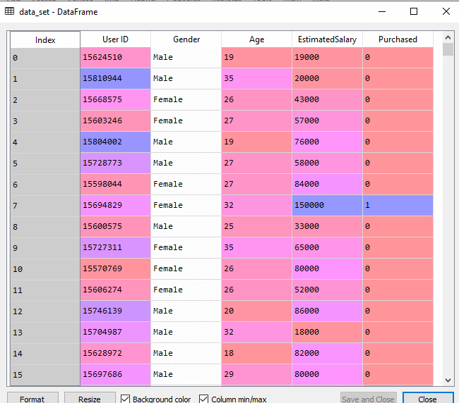
2. Fitting a Decision-Tree algorithm to the Training set

Now we will fit the model to the training set. For this, we will import the DecisionTreeClassifier class from sklearn.tree library. Below is the code for it:

1. #Fitting Decision Tree classifier to the training set  
2. From sklearn.tree import DecisionTreeClassifier  
3. Classifier= DecisionTreeClassifier(criterion='entropy', random_state=0)  
4. Classifier.fit(x_train, y_train)  

In the above code, we have created a classifier object, in which we have passed two main parameters;

• "criterion='entropy': Criterion is used to measure the quality of split, which is calculated by information gain given by entropy.
• Random_state=0": For generating the random states.

Below is the output for this:

Out[8]:

DecisionTreeClassifier(class_weight=None, criterion='entropy', max_depth=None,

Max_features=None, max_leaf_nodes=None,

Min_impurity_decrease=0.0, min_impurity_split=None,

Min_samples_leaf=1, min_samples_split=2,

Min_weight_fraction_leaf=0.0, presort=False,

                       random_state=0, splitter='best')

3. Predicting the test result

Now we will predict the test set result. We will create a new prediction vector y_pred. Below is the code for it:

1. #Predicting the test set result  
2. y_pred= classifier.predict(x_test)  

Output:

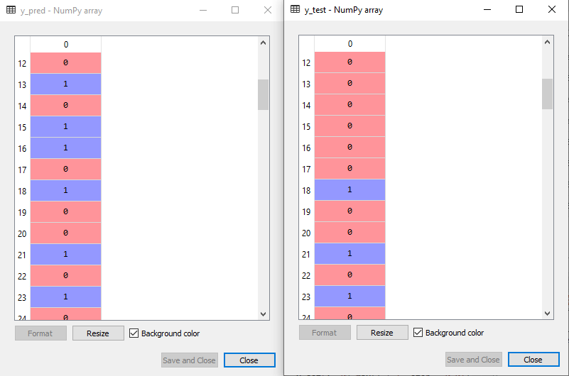
In the below output image, the predicted output and real test output are given. We can clearly see that there are some values in the prediction vector, which are different from the real vector values. These are prediction errors.

4. Test accuracy of the result (Creation of Confusion matrix)

In the above output, we have seen that there were some incorrect predictions, so if we want to know the number of correct and incorrect predictions, we need to use the confusion matrix. Below is the code for it:

1. #Creating the Confusion matrix  
2. From sklearn.metrics import confusion_matrix  
3. Cm= confusion_matrix(y_test, y_pred)  

Output:

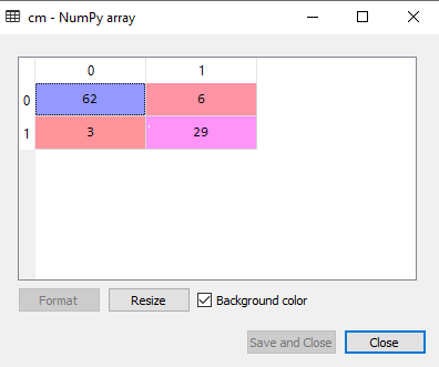
In the above output image, we can see the confusion matrix, which has 6+3= 9 incorrect predictions and62+29=91 correct predictions. Therefore, we can say that compared to other classification models, the Decision Tree classifier made a good prediction.

5. Visualizing the training set result:

Here we will visualize the training set result. To visualize the training set result we will plot a graph for the decision tree classifier. The classifier will predict yes or No for the users who have either Purchased or Not purchased the SUV car as we did in Logistic Regression. Below is the code for it:

1. #Visulaizing the trianing set result  
2. From matplotlib.colors import ListedColormap  
3. x_set, y_set = x_train, y_train  
4. x1, x2 = nm.meshgrid(nm.arange(start = x_set[:, 0].min() - 1, stop = x_set[:, 0].max() + 1, step  =0.01),  
5. Nm.arange(start = x_set[:, 1].min() - 1, stop = x_set[:, 1].max() + 1, step = 0.01))  
6. Mtp.contourf(x1, x2, classifier.predict(nm.array([x1.ravel(), x2.ravel()]).T).reshape(x1.shape),  
7. Alpha = 0.75, cmap = ListedColormap(('purple','green' )))  
8. Mtp.xlim(x1.min(), x1.max())  
9. Mtp.ylim(x2.min(), x2.max())  
10. Fori, j in enumerate(nm.unique(y_set)):  
11. Mtp.scatter(x_set[y_set == j, 0], x_set[y_set == j, 1],  
12.        c = ListedColormap(('purple', 'green'))(i), label = j)  
13. Mtp.title('Decision Tree Algorithm (Training set)')  
14. Mtp.xlabel('Age')  
15. Mtp.ylabel('Estimated Salary')  
16. Mtp.legend()  
17. Mtp.show()  

Output:

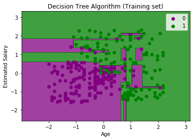
The above output is completely different from the rest classification models. It has both vertical and horizontal lines that are splitting the dataset according to the age and estimated salary variable.

As we can see, the tree is trying to capture each dataset, which is the case of overfitting.

6. Visualizing the test set result:

Visualization of test set result will be similar to the visualization of the training set except that the training set will be replaced with the test set.

1. #Visulaizing the test set result  
2. From matplotlib.colors import ListedColormap  
3. x_set, y_set = x_test, y_test  
4. x1, x2 = nm.meshgrid(nm.arange(start = x_set[:, 0].min() - 1, stop = x_set[:, 0].max() + 1, step  =0.01),  
5. Nm.arange(start = x_set[:, 1].min() - 1, stop = x_set[:, 1].max() + 1, step = 0.01))  
6. Mtp.contourf(x1, x2, classifier.predict(nm.array([x1.ravel(), x2.ravel()]).T).reshape(x1.shape),  
7. Alpha = 0.75, cmap = ListedColormap(('purple','green' )))  
8. Mtp.xlim(x1.min(), x1.max())  
9. Mtp.ylim(x2.min(), x2.max())  
10. Fori, j in enumerate(nm.unique(y_set)):  
11. Mtp.scatter(x_set[y_set == j, 0], x_set[y_set == j, 1],  
12.        c = ListedColormap(('purple', 'green'))(i), label = j)  
13. Mtp.title('Decision Tree Algorithm(Test set)')  
14. Mtp.xlabel('Age')  
15. Mtp.ylabel('Estimated Salary')  
16. Mtp.legend()  
17. Mtp.show()  

Output:

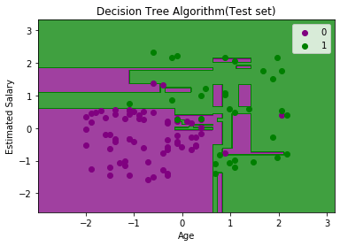
As we can see in the above image that there are some green data points within the purple region and vice versa. So, these are the incorrect predictions which we have discussed in the confusion matrix.

9.     What are Artificial Neural Networks (ANNs)?

The inventor of the first neurocomputer, Dr. Robert Hecht-Nielsen, defines a neural network as −

"...a computing system made up of a number of simple, highly interconnected processing elements, which process information by their dynamic state response to external inputs.”

Basic Structure of ANNs

The idea of ANNs is based on the belief that working of human brain by making the right connections, can be imitated using silicon and wires as living neurons and dendrites.

The human brain is composed of 86 billion nerve cells called neurons. They are connected to other thousand cells by Axons. Stimuli from external environment or inputs from sensory organs are accepted by dendrites. These inputs create electric impulses, which quickly travel through the neural network. A neuron can then send the message to other neuron to handle the issue or does not send it forward.

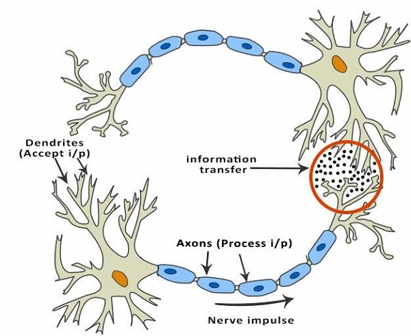
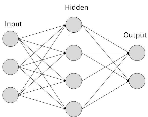
ANNs are composed of multiple nodes, which imitate biological neurons of human brain. The neurons are connected by links and they interact with each other. The nodes can take input data and perform simple operations on the data. The result of these operations is passed to other neurons. The output at each node is called its activation or node value.

Each link is associated with weight. ANNs are capable of learning, which takes place by altering weight values. The following illustration shows a simple ANN −

Types of Artificial Neural Networks

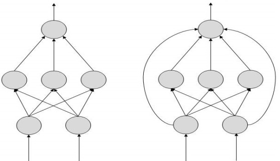
There are two Artificial Neural Network topologies − FeedForward and Feedback.

FeedForward ANN

In this ANN, the information flow is unidirectional. A unit sends information to other unit from which it does not receive any information. There are no feedback loops. They are used in pattern generation/recognition/classification. They have fixed inputs and outputs.

FeedBack ANN

Here, feedback loops are allowed. They are used in content addressable memories.

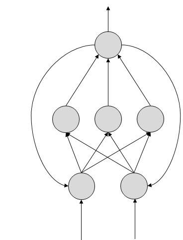
Working of ANNs

In the topology diagrams shown, each arrow represents a connection between two neurons and indicates the pathway for the flow of information. Each connection has a weight, an integer number that controls the signal between the two neurons.

If the network generates a “good or desired” output, there is no need to adjust the weights. However, if the network generates a “poor or undesired” output or an error, then the system alters the weights in order to improve subsequent results.

10. Write some of the Applications of Neural Networks

They can perform tasks that are easy for a human but difficult for a machine −

• Aerospace − Autopilot aircrafts, aircraft fault detection.
• Automotive − Automobile guidance systems.
• Military − Weapon orientation and steering, target tracking, object discrimination, facial recognition, signal/image identification.
• Electronics − Code sequence prediction, IC chip layout, chip failure analysis, machine vision, voice synthesis.
• Financial − Real estate appraisal, loan advisor, mortgage screening, corporate bond rating, portfolio trading program, corporate financial analysis, currency value prediction, document readers, credit application evaluators.
• Industrial − Manufacturing process control, product design and analysis, quality inspection systems, welding quality analysis, paper quality prediction, chemical product design analysis, dynamic modeling of chemical process systems, machine maintenance analysis, project bidding, planning, and management.
• Medical − Cancer cell analysis, EEG and ECG analysis, prosthetic design, transplant time optimizer.
• Speech − Speech recognition, speech classification, text to speech conversion.
• Telecommunications − Image and data compression, automated information services, real-time spoken language translation.
• Transportation − Truck Brake system diagnosis, vehicle scheduling, routing systems.
• Software − Pattern Recognition in facial recognition, optical character recognition, etc.
• Time Series Prediction − ANNs are used to make predictions on stocks and natural calamities.
• Signal Processing − Neural networks can be trained to process an audio signal and filter it appropriately in the hearing aids.
• Control − ANNs are often used to make steering decisions of physical vehicles.
• Anomaly Detection − As ANNs are expert at recognizing patterns, they can also be trained to generate an output when something unusual occurs that misfits the pattern.