undefined | unit 2 statistical decision theory

Back to Study material

Unit-2 Statistical Decision Theory Q1) What is linear regression?A1) Linear Regression Simple linear regression is a regression method in which the independent variable and the dependent variable have a linear relationship. In the diagram, the straight line is the best fit line. The main objective of simple linear regression is to take into account the given data points and plot the best fit line to best fit the model.

Fig 1: linear regression The basic algorithm for evaluating the linear relationship between the target variable and the input features is believed to be linear regression. The green dots in the above picture represent the actual values, while the red line represents the regression line that was applied to the actual data. The line equation is used to populate the equation.Y = mX + c Where,

● Y is the predicted value,

● X is feature value,

● m is coefficients or weights,

● c is the bias value.

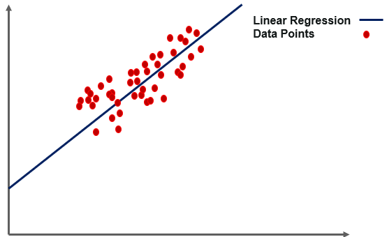
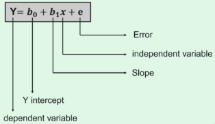
Usage Cases for Linear Regression ● Revenue Forecasting● Risk Evaluation● Applications for Housing To Forecast Prices and Other Factors● Stock price forecasting, investment assessment, and other finance applications The basic concept behind linear regression is to figure out how the dependent and independent variables are related. It's used to find the best-fitting line that can correctly predict the result with the least amount of error. We may use linear regression in simple real-life scenarios, such as predicting SAT scores based on study hours and other important factors. Basic Terminology it's important to understand the following words : Cost function
The linear equation given below can be used to find the best fit line.

● Y stands for the dependent variable that needs to be expected.

● The intercept b0 denotes a line that touches the y-axis.

● The slope of the line is b1, and the independent variables that decide the prediction of Y are represented by x.

● The error in the final forecast is denoted by the letter e.

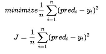
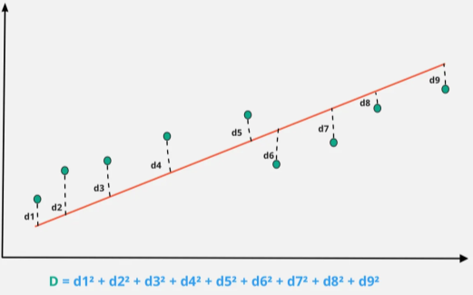
The cost function determines the best possible values for b0 and b1 in order to construct the best possible fit line for the data points. To get the best values for b0 and b1, we turn this problem into a minimization problem.

We select these functions for minimizing the error. Gradient DescentGradient descent is the next significant concept to learn in order to understand linear regression. It is a method of lowering the MSE by modifying the b0 and b1 values. The target is to keep iterating the b0 and b1 values until the MSE is as low as possible. We use the gradients from the cost function to change b0 and b1. We use partial derivatives with respect to b0 and b1 to find these gradients. The gradients are the partial derivatives that are used to change the values of b0 and b1.

Fig 2: gradient descent Q2) Write the advantages and disadvantages of linear regression?A2) Advantages of linear regression ● For linearly separable data, linear regression performs exceptionally well.● It's simpler to introduce, interpret, and practice with.● It uses dimensionality reduction methods, regularization, and cross-validation to effectively tackle overfitting.● Extrapolation beyond a single data set is another benefit. Disadvantages of linear regression ● The belief that dependent and independent variables are linear● It's susceptible to a lot of noise and overfitting.● Outliers are very sensitive to linear regression.● Multicollinearity is a concern. Q3) Explain ridge regression?A3) Ridge Regression Ridge regression is a model tuning technique that can be used to evaluate data with measurement errors. L2 regularization is accomplished using this approach. Where there is a problem with multicollinearity, least-squares are unbiased, and variances are high, the expected values are far from the actual values. The ridge regression cost function is as follows: Min(||Y – X(theta)||^2 + λ||theta||^2) The penalty word is lambda. The ridge function's alpha parameter denotes the value given here. We can regulate the penalty term by adjusting the values of alpha. The higher the alpha value, the greater the penalty, and thus the magnitude of the coefficients is decreased. ● It decreases the size of the parameters. As a result, it's used to avoid measurement errors.● It uses coefficient shrinkage to reduce the model's complexity. Ridge regression model The basic regression equation serves as the basis for any form of regression machine learning model, and it is written as: Y = XB + e The dependent variable is Y, the independent variables are X, the regression coefficients to be calculated are B, and the errors are residuals are e. The variance that is not measured by the general model is taken into account when the lambda function is applied to this equation. There are measures that can be taken after the data has been prepared and marked as being part of the L2 regularization process. Bias and Variance When it comes to constructing ridge regression models on a real dataset, the trade-off between bias and variance is typically difficult. However, the following is a general pattern to bear in mind: ● When it rises, the prejudice rises with it.● As increases, the variance decreases. The term bias refers to the degree to which the model fails to generate a plot that is consistent with the samples, rather than the y-intercept.

Fig 3: bias Contrary to common opinion, variance does not refer to the distribution of data, but rather to how a model's accuracy varies across different datasets.

Fig 4: variance Ridge regression is almost similar to linear regression (sum of squares), with the exception that a small amount of bias is added. We get a major reduction in variance as a result. Ridge Regression, in other words, may provide better long-term forecasts by beginning with a slightly worse fit.The Ridge Regression penalty is the bias that is applied to the model. Lambda is multiplied by the squared weight of each individual function to get it. Q4) Define lasso?A4) LassoLeast Absolute Shrinkage and Selection Operator (LASSO) is an acronym for Least Absolute Shrinkage and Selection Operator. Lasso regression is a form of regularization. For a more precise forecast, it is favoured over regression approaches. Shrinkage is used in this model. Data values are shrunk towards a central point known as the mean in shrinkage. Easy, sparse models are encouraged by the lasso technique (i.e. models with fewer parameters). This method of regression is suitable for models with a lot of multicollinearity or when you want to automate parts of the model selection process, such as variable selection and parameter elimination. The L1 regularization technique is used in Lasso Regression. It is used when there are a large number of features because it performs feature selection automatically. Lasso regression performs L1 regularization, which means it applies a dimension to the optimization goal equal to the number of absolute values of coefficients. As a result, lasso regression increases the following: Objective = RSS + α * (sum of absolute value of coefficients) In this case, (alpha) functions similarly to ridge and offers a trade-off between balancing RSS and coefficient magnitude. Similarly to ridge, may have a number of values.

Let's go over it again quickly:

● α = 0: Same coefficients as simple linear regression

● α = ∞: All coefficients zero

● 0 < α < ∞: coefficients between 0 and that of simple linear regression.

The RSS plus the sum of absolute values of weight magnitudes is the objective function (also known as the cost) to be minimized. Mathematically, this can be expressed as:

Fig 5: Statistics of lasso regression

d1, d2, d3, etc represents the distance between the actual data points and the model line. Q5) What do you mean by principal component analysis?A5) Principal Component AnalysisPrincipal Component Analysis is a feature extraction process in which we generate new independent features from old features and retain only the features that are most relevant in predicting the target from the combination of both. New features are derived from old features, and any function that is less reliant on the target variable can be dropped. Principal Component Analysis (PCA) is a common technique for reducing the dimensionality of a large data set. Reducing the number of components or features compromises some precision, but it simplifies, examines, and visualizes a broad data set. It also reduces the model's computational complexity, allowing machine learning algorithms to run faster. It is still a challenge and a point of contention as to how much precision is lost in order to achieve a less complex and reduced-dimension data set. We don't have a fixed answer for this, but when selecting the final set of components, we try to retain as much variation as possible. Steps involved in PCA● Ensure that the data is standardized. (where the mean is 0 and the variance is 1)● Calculate the dimension's covariance matrix.● From the covariance matrix, obtain the Eigenvectors and Eigenvalues (we can also use correlation matrix or even Single value decomposition).● Choose the top k Eigenvectors that correspond to the k largest eigenvalues (k will become the number of dimensions of the new function subspace kd, d is the number of original dimensions) by sorting eigenvalues in descending order.● Create the projection matrix W using the k Eigenvectors you've chosen.● To get the new k-dimensional function subspace Y, transform the original data set X through W. Performance issues ● PCA's potency is directly proportional to the scale of the attributes. If the variables are on different scales, PCA will choose the one with the highest attributes without regard for correlation.● If the scale of a variable is changed, PCA can change.● PCA can be difficult to interpret due to the presence of discrete data.● The appearance of skew in the data with long thick tails can affect the effectiveness of PCA.● When the relationships between attributes are not linear, PCA is ineffective. Q6) What do you mean by partial least squares?A6) Partial Least SquarePLS, or Partial Least Squares, is a common regression technique for analyzing data from near-infrared spectroscopy. One potential downside of PCR is that we cannot be certain that the selected principal components are connected to the outcome. The outcome variable does not supervise the selection of the principal components to use in the model in this scenario.The Partial Least Squares (PLS) regression is an alternative to PCR in that it discovers new principal components that not only summarize the original predictors but also are linked to the outcome. The regression model is then fitted using these components. In comparison to PCR, PLS implements a dimension reduction approach that is overseen by the result. PLS, like PCR, works well with data that has strongly correlated predictors. Cross-validation is widely used to evaluate the number of PCs used in PLS. To make the variables comparable, predictors and outcome variables should be standardized in general. PLS is a dimension reduction approach that implements the same method as concept components regression, but it selects new predictors (principal components) in a supervised manner. The PLS method searches for instructions (i.e., principal components) that can help explain both: ● the answer, ● as well as the initial predictors PLS looks for a shift in the original predictors that is also relevant to the answer. Q7) Write the advantages and disadvantages of principal component analysis?A7) Advantages of principal component analysis ● Due to the orthogonal elements, there is a lack of data redundancy.● Noise reduction due to the use of the maximum variance basis, which automatically eliminates minor variations in the context. Disadvantages of principal component analysis ● It's difficult to do a thorough assessment of covariance.● The PCA would not be able to capture even the most basic invariance unless the training data specifically provided this detail. Q8) Write about ML?A8) MLBayesian Machine Learning (Bayesian ML) is a method for creating mathematical models based on Bayes' Theorem.

The aim of Bayesian machine learning is to estimate the posterior distribution ( p(θ|x) ) provided the probability ( p(x|θ) ) and the prior distribution, p(θ). The probability is a number that can be determined based on the training data. Consider the probability that our code is bug-free. Our code is bug-free and passes all test cases, as shown by and X, respectively. ● P(θ) – The probability of the hypothesis being true before applying the Bayes' theorem is known as prior probability. Prior refers to either common sense or an outcome of Bayes' theorem for certain previous findings, and it reflects the values that we have learned from past experience. Prior chance, in this case, refers to the possibility of finding no bugs in our code. However, since this is the first time we've used Bayes' theorem, we'll have to come up with other ways to evaluate the priors (otherwise we could use the previous posterior as the new prior). We may allocate a higher probability to our prior P(θ). For the time being, let us assume that P(θ) = p. ● P(X|θ) – The conditional probability of the evidence given a hypothesis is called likelihood. The probability is primarily calculated by our observations or data. If we conclude that our code is bug-free, the likelihood is the probability of our code passing all test cases. Assuming we've implemented these test cases right, if our code doesn't contain any bugs, it should pass all of them. Therefore, the likelihood P(X|θ) = 1. ● P (X) – Evidence term denotes the probability of evidence or data. This can be expressed as a summation (or integral) of the probabilities of all possible hypotheses weighted by the likelihood of the same.

As a consequence, P(X) can be written as:

We write P(X) as an integration for the continuous:

Q9) Write about MAP ?A9) MAP (Maximum a Posteriori)While MAP is the first step toward completely Bayesian machine learning, it still only computes a point estimate, which is an estimate for the value of a parameter at a single point based on data. Point estimates have the drawback of not telling you anything about a parameter other than its optimum setting. In fact, we always want to know more information, such as how sure we are that the value of a parameter will fall within this predefined range. To that end, Bayesian ML's true strength lies in computing the entire posterior distribution. However, this is a tricky business. Distributions aren't tidy mathematical objects that can be fiddled with at will. They're frequently defined as complicated, intractable integrals over continuous parameter spaces that are impossible to compute analytically. As a consequence, a variety of fascinating Bayesian methods for sampling (i.e. drawing sample values) from the posterior distribution have been established. From a set of theories, we can use MAP to find the most probable one. According to MAP, the hypothesis with the highest posterior likelihood is the most likely to be correct. As a consequence, the hypothesis MAP that is concluded using MAP can be represented as follows:

The argmaxθ operator calculates the likelihood of an occurrence or hypothesis θi that maximizes the posterior probability P(θi|X). Let's use MAP to find out what the true hypothesis is in the above example:

The figure depicts how the posterior probabilities of potential hypotheses shift as the prior probability increases.

Fig 7: P(X|θ) and P(X|¬θ) when changing the P(θ) = p Q10) What do you mean by conjugate priors ?A10) Conjugate Priors

We've estimated our posterior for, but even more impressive, we've returned to the Gamma distribution! Let's take a look at how this works. The gamma distribution is defined as follows:

We chose values for k and quite haphazardly at the start of this article. Now note that if we choose k = 10 and = 0.5, we get our posterior!

that simply implies that we choose C in our posterior calculation:

● The Bayesian framework offers simple solutions to a variety of difficult problems, ○ such as estimating uncertainty, selecting multiple hyper-parameters, and dealing with non-IID results. ● However, it often necessitates:○ the representation of high-dimensional distributions.○ Solving problems concerning high-dimensional integration. ● We've seen it work in a few unusual situations:○ With a discrete prior, Bernoulli probability yields discrete posterior (0.5 or 1).○ When Bernoulli probability is paired with a beta prior, the outcome is beta posterior.○ Gaussian posterior is obtained by combining Gaussian probability with Gaussian prior (linear regression). ● These are simple since the posterior belongs to the same ‘family' as the prior:○ this is known as a conjugate probability prior. ● The basic definition of conjugate priors is as follows:x ∼ D(θ), θ ∼ P(λ) ⇒ θ | x ∼ P(λ 0 ). ● Example of Beta-bernoulli:x ∼ Ber(θ), θ ∼ B(α, β), ⇒ θ | x ∼ B(α’ , β’ )Specifically, if we see h heads and t tails, the posterior is B(h +α, t + β). ● Example of Gaussian-Gaussian:x ∼ N (µ, Σ), µ ∼ N (µ0, Σ0), ⇒ µ | x ∼ N (µ’ , Σ’)and the posterior predictive is a Gaussian as well. ● If is a random variable, then:○ Wishart's conjugate prior is natural - inverse.○ A student t is posterior predictive.

Sign Up