Unit – 5
Scalar Quantization of LPC
Q1) What are spectral distortion measures?
Ans: Spectral distortion measures
The aim of a spectral sensitivity function is to measure the magnitude change in spectral distortion caused by changing one of the PSDs defining parameters.
Given two sets of LPCs a1,i and a2,i , i = 1, 2, ... , M, we define the polynomials

The prediction order is denoted by the letter M. The machine functions of two AR process analyzers with different parameters are represented by the polynomials above. Thus, assuming unit variance input white noise, the PSDs of the two AR signals shown above are

Between S1 and S2, the spectral distortion is defined by

where the result is represented in decibels directly In other words, if fs is the sampling frequency, we get

In fact, the integrals in above two equations can be approximated by sampling the PSDs with N points:

where 0 ≤ n0 ≤ n1 ≤ N is the number of the number of the number of the number of the number of the number of the number of the number of the number of the number of For fs = 8 kHz, n0 = 4, n1 = 100, and N = 256, respectively, so that only the spectrum values between 125 Hz and approximately 3.1 kHz are used to compute SD. As a result, only the most perceptually receptive portion of the spectrum is taken into account.
Q2) Explain requirements of Transparent quantization of LP?
Ans: Requirements for Transparent Quantization of LP
By ‘‘transparent," we say that the LPC quantization causes no audible distortion in the coded speech; in other words, two versions of coded speech—one obtained with an unquantized LPC and the other obtained with a quantized LPC—are indistinguishable via listening.
The average spectral distortion has been widely used to assess LPC quantizer efficiency. For example,1 dB average SD has been found to be a satisfactory limit for transparent quantization. The quantizer is said to have achieved transparent quantization if the average SD is less than 1 dB.
The quantizer is said to have achieved transparent quantization if the average SD is less than 1 dB. However, even though the average SD is 1 dB, it has been found that too many outlier frames with large SD in a speech utterance can cause audible distortion. As a result, lowering both the average SD and the number of outlier frames is highly desirable. The conditions mentioned below are good starting points for transparent quantification.
● A spectral distortion of less than 1 dB on average.
● Spectral distortion greater than 2 dB is seen in less than 2% of outliers.
● There were no outliers of spectral distortion greater than 4 decibels.
Spectral Sensitivity Function
Consider the S(ejw , x) power spectral density, which is a function of both the frequency o and the parameter x. The PSD is regulated by the parameter x, which in this case may be one of the LPCs or another related variable. The function can be used to consider the effect of changing one parameter on spectral distortion.

The spectral sensitivity function, also known as the spectral sensitivity function, is defined. In the above equation, spectral distortion (SD) is written as

As a result, the spectral sensitivity function determines the degree of change in spectral distortion caused by a change in one of the PSDs defining parameters.

Fig 1: Examples of spectral sensitivity curves with respect to reflection coefficient
Q3) Describe Quantization based on reflection coefficient?
Ans: Each parameter or its alternative form is quantized independently of the others in scalar quantization of the LPC. We can see from the description of SD that it is a function of all the parameters.
As a result, scalar quantization applied to the LPC is suboptimal in terms of SD, in the sense that when a parameter is quantized separately, SD is not minimized in the best possible way. Scalar quantization, on the other hand, is used in a variety of speech coding standards due to its simplicity.
The coefficient to be quantized is compared to a codebook where the quantized values, or codewords, are stored in a scalar quantization scheme. The quantized coefficient is chosen as the codeword that is nearest to the coefficient, with the distance measured by the squared difference. As a result, the average spectral distortion will decrease as the codebook sizes for different coefficients increase.
In practice, using a collection of test results, it is possible to evaluate the quantizers' outputs at various resolutions and choose the ones that provide a low enough average SD to satisfy the transparent quantization requirements. The Lloyd algorithm can be used to construct the codebooks, which uses a collection of training data to minimize the amount of squared error.
The reflection coefficient is a strong candidate for quantization since the magnitude can easily verify the synthesis filter's stability. A collection of training coefficients obtained from a speech database is thus used to design an RC-based LPC scalar quantizer. To obtain the resultant codebooks, the Lloyd algorithm is used.
When the magnitudes of the coefficients are similar to one, the spectral sensitivity functions for the RC appear to have high values, which is an issue with the design process. As the magnitudes of the coefficients exceed one, this causes difficulties, making it impossible to meet the straightforward quantization criteria.
When the magnitudes of the coefficients are near one, a quantizer that is much more sensitive (smaller phase size) than when they are near zero is needed. That is, the quantizer's transfer characteristic is non uniform. The use of a non uniform quantizer is equivalent to uniform quantization of a transformed coefficient through a nonlinear function; in other words,
g = f(k)
where k denotes the reflection coefficient, f(.) denotes a nonlinear function, and g denotes the transformed coefficient value. The nonlinear function's necessary form is depicted in the diagram.

Fig 2: Illustration of a nonlinear mapping applied to reflection coefficients
It's worth noting that uniform quantization intervals on the vertical axis (g) result in nonuniform intervals on the horizontal axis (k), with the horizontal intervals becoming shorter as the magnitude of the input coefficient reaches one. As a result, reflection coefficients with magnitudes close to one are more susceptible to the quantizer.
Viswanathan and Makhoul (1975) proposed the function

which can be seen in Figure. The function, as can be shown, meets the quantization requirements. The log area ratio is the product of the RC transformation (LAR).

Fig 3: Nonlinear function associated with the log area ratio. The identity line is superimposed
The word "area ratio" comes from the RC's connection to the acoustic tube model for speech output, in which the tube areas are proportional to the coefficients. With g = f(k), the inverse relationship is
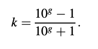
Above figure shows a comparison of the nonlinear function and the identity function. The LAR curve is almost linear for values of k less than 0.7 in magnitude. As a result, if the magnitude of a given RC has a high probability of being less than 0.7, the quantization efficiency of a uniform quantizer in the RC and LAR domains is comparable. In reality, RCs with orders greater than three (k1; I > 3) have magnitudes less than 0.7 in general. This reality can be used to build a quantizer.
Q4) Describe Bit Allocation?
Ans: Bit allocation
It is not advisable to use an equivalent number of bits for the quantization of different parameters in a scalar quantization scheme where each coefficient or parameter is quantized separately, since each parameter contributes differently to the average spectral distortion.
When a collection of training data is available, the following technique can be used to optimize the bit allocation process during the actual design of a scalar quantizer.
When a quantizer provides the lowest average spectral distortion, the process assigns one bit to it and iterates until the appropriate number of bits is reached. The final results are determined by the training data set; bit allocation for various parameters is generally nonuniform.
Step 1 : Initialization: Set m = 0. Begin with a resolution of r0 = 0. All quantizer mapping functions are zero; in other words,
Qm,l(x) = Q0,l(x) = 0; l = 1, 2, ... , M.
Step 2 : Make m ← m + 1 Increase the amount of bits allotted by 1:
rm = rm-l + 1
Stop rm if it exceeds the amount of bits available.
Step 3 : For l = 1, 2, ... , M:
● Create a quantizer Qm,l(x) with a resolution of rm,l = rm-1,l + 1.
● Find the average spectral distortion SDm,l using Qm,l(x) and Qm-1,n (x), n ≠ l.
Step 4 : Choose the index l so that SDm,l is as small as possible. The quantizers for the mth iteration are then applied.
Qm,l(x),
Qm,n(x) = Qm-l,n(x), n ≠ l:
Return to Step 2.
The method described above is known as greedy because the solution is always chosen from the one that appears to be the best at the time. That is, it allows a locally optimal decision in the hopes of achieving a globally optimal result. Greedy algorithms do not always produce optimal solutions, but they are used to solve many practical optimization problems due to their simplicity.
TIA IS54 VSELP
To capture the spectral envelope, this algorithm uses a frame length of 160 samples (20 ms) and a prediction order of 10. The ten RCs k1 to k10 are quantized using 6, 5, 5, 4, 3, 3, 3, 3, 2, and 2 bits, for a total of 38 bits per frame. The quantizers' resolution is reduced for higher-order coefficients because they are less essential for the spectrum's description. The cost of the LAR computation is eliminated by directly quantifying the RC.
ETSI GSM 6.10 RPE-LTP
This coder uses a prediction order of 8 and has a frame length of 160 samples (20 ms). A piecewise linear function is used to convert the RC to the LAR. Different uniform quantizers with different limits are used due to their different dynamic ranges and amplitude distributions. The resolutions of the quantizers will gradually decrease as the order increases because spectral distortion becomes less dependent on higher-order coefficients. The eight LARs g1 to g8 are quantized with 6, 6, 5, 5, 4, 4, 3, and 3 bits, for a total of 36 bits per frame.
FS1015 LPC
This coder uses a frame length of 180 samples (22.5 ms) and classifies each frame as voiced or unvoiced based on the frame's periodicity. For voiced frames, a tenth-order predictor is used, but for unvoiced frames, only a fourth-order predictor is used. This is achieved since a lower-order predictor is adequate to characterize the spectral envelope for unvoiced frames.
Scalar quantization is used in both the LAR and RC domains to quantify the LPC. Table summarizes the bit allocation method. Only the first two parameters are quantized in the LAR domain, as can be shown. This is because only the first two RCs have a statistically important chance of getting magnitudes equal to one.
Table : Bit Allocation for LPC Quantization of the FS1015 Coder
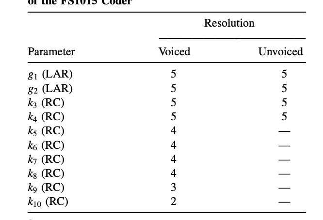
The benefit of limiting LAR quantization to the first two coefficients is that it saves time. For all quantizers, uniform quantization is used. The LPC information is transmitted at a limit of 41 bits per frame.
Q5) What do you mean by Line spectral frequency – LPC to LSF conversions?
Ans: Itakura (1975) was the first to propose line spectral frequency (LSF) as an alternative representation of LPC. The LSF has gained widespread acceptance in speech coding applications due to its many desirable properties.
LPC-to-LSF Conversion
The aim is to convert the set of LPCs ai, I = 1,..., M into the alternative LSF representation, denoted by ωi,i = 1,..., M, with 0 < ωi < π . The steps are outlined below.
● Find the polynomial coefficients.
For M even: M1 = M2 = M = 2:
For M odd: M1 = (M + 1)/2, M2 = (M - 1)/2
pi = ai + aM-i+1; i = 1, ... , M1,
qi = ai - aM-i+1; i = 1, ... , M2,
p0’ = 1;
pi’ = pi - p’i-1; i = 1, ... , M
For M even:

For M odd:

● Construct the functions Po(ω) and Qo(ω) and solve for roots, that is, the frequency values when Po(ω) = 0 or Qo(ω) = 0 for 0 < ω < p. The LSFs are the frequency values.
It's worth noting that the functions Po(ω) and Qo(ω) are order-dependent and must be sought for each order of interest. The functions are derived, for example, for the widely used value of M = 10. The cosine measurement is relatively costly to implement in a realistic setting. As a result, it is easy to use the substitution x = cos(ω) so that the root values in x are found first while root solving. The LSFs are provided by denoting the roots as xi.
oi = cos-1 (xi)
The substitution x = cos(ω) is used to rewrite the two frequency functions for M = 10.
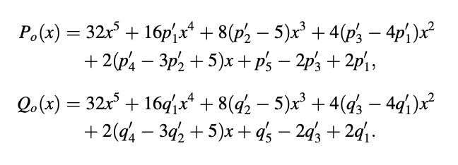
Example 1: Following the LPC to LSF conversion protocol, the coefficients are as follows:

The frequency functions that result are as follows:

Figure 5 depicts these functions, with the LSF values deduced from the intersections with the frequency axis. The equivalent functions are plotted in Figure 6 using the mapping x = cos(ω), with -1 < x < 1. The LSFs that result are found to be

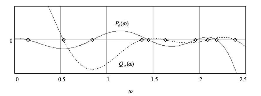
Fig 4: Plot of some example frequency functions. LSF values are marked on the horizontal axis
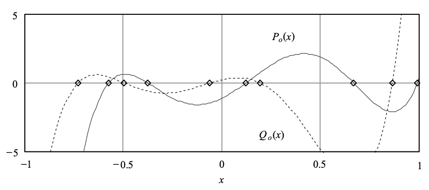
Fig 5: Plot of some example frequency functions with x = cos(ω)
The odd-indexed parameters are from Qo(ω), while ω1, ω3, ω5, ω7 and ω9 are from Po(ω). This example demonstrates a significant property of the LSF: the zeros of Po(ω) and Qo(ω) are interlaced with each other, in the way that the zeros of Po(ω) and Qo(ω) are interlaced with each other.
ω1 > ω2 > ω3, >……….. > ω10
As long as the LPCs are from a minimum-phase device, this property is satisfied.
Q6) Explain Quantization based on LSF?
Ans: First, as long as the interlacing condition is met, the related synthesis filter's minimum-phase property is retained after quantization. The values of the LSFs, on the other hand, regulate the frequency domain property of the signal, and changes in one parameter have a local effect on the spectrum. The LSFs are also bounded: they fall within the (0, π) interval, making them ideal for fixed-point implementation.
The LSF allows the synthesis filter's stability to be easily controlled, as well as the amount of distortion in each frequency region. Interpolation has also been found to benefit from the use of the LSF.
The LSF is first found in the cosine domain x = cos(ω), x ∈ [-1, 1] and later is mapped to the frequency domain ω = cos-1(x), ω ∈ [0,π] . The parameters are often explicitly quantized in the cosine domain for quantization purposes, since the mapping using cos-1 requires extra computation, and the interlacing property can be checked in both domains.
FS1016 CELP
A frame length of 240 samples is used in this algorithm (30 ms). An LP review of the tenth order is carried out. Ten separate non uniform quantizers are used to quantify the LPCs as LSFs. In Figure, the codewords are summarized. Since the frequency range protected by these four parameters is the most sensitive for a human audience, more bits are reserved for the second to fifth parameters. The ten LSFs ω1 to ω10 are quantized using 3, 4, 4, 4, 4, 3, 3, 3, 3, and 3 bits, respectively, leading to a total of 34 bits/frame.

Fig 6: Plot of LSF quantization codewords for the FS1016 coder
Conversion of LPC to Quantized LSF
The codewords are denoted by fi,j in the LPC quantizer of the FS1016 CELP coder, where i = 1 to 10 indicates the quantizer number; and j = 1 to 𝛼i indicates the codeword number, with 𝛼i 1= 8 for i = 1 and i = 6 to 10, and 𝛼i = 16 for i = 2 to 5. These codewords are first translated into English.

The root function for converting the LPC to the LSF, can be simplified since the final LSF values are fixed and known: they are already shown in the above Figure . As a result, the table's availability means a reduction in computation time during the LPC-to-LSF conversion. Figure shows the flowchart of the new root routine; however, in this case, the quantizer's index, I is passed to the routine as an input parameter.

Fig 7: Flowchart of the root function, applicable when the quantized LSF values are known.
The function form (P or Q), the initial search value x, and the quantizer index I are all input parameters in this routine. The codeword that is only smaller than the initial search value x is calculated in the first loop. The next loop looks for a sign shift by going through the remaining codewords one by one. The routine is clearly simpler than and has a lower level of difficulty.
Q7) What are the advantages of vector quantization over scalar quantization?
Ans: Advantages of vector quantization over scalar quantization
● With the number of reconstruction levels kept constant, Vector Quantization can reduce average distortion, while Scalar Quantization cannot.
● When distortion is constant, Vector Quantization can reduce the number of reconstruction stages, while Scalar Quantization cannot.
● The statistical dependency among scalars in the block is the most significant way Vector Quantization can improve performance over Scalar Quantization.
● In addition, Vector Quantization is more efficient than Scalar Quantization. When the output values from the source are not correlated.
● In comparison to Scalar Quantization, Vector Quantization offers more versatility in terms of modifications. With increasing dimensions, Vector Quantization becomes more flexible in terms of change.
● When there is sample to sample dependency of data, Vector Quantization performs better than Scalar Quantization.
● When there is no sample to sample dependency of the input, Vector Quantization performs better than Scalar Quantization.
● The Granular Error in Scalar Quantization is only affected by the size of the quantization interval, while the Granular Error in Vector Quantization is affected by both the form and the size of the quantization interval.
Q8) Write the difference between scalar quantization and vector quantization?
Ans: Difference between scalar quantization and vector quantization
2. When distortion is constant, Vector Quantization can reduce the number of reconstruction stages, while Scalar Quantization cannot.
3. The statistical dependency among scalars in the block is the most significant way Vector Quantization can improve performance over Scalar Quantization.
4. In addition, Vector Quantization is more efficient than Scalar Quantization. When the output values from the source are not correlated.
5. In comparison to Scalar Quantization, Vector Quantization offers more versatility in terms of modifications. With increasing dimensions, Vector Quantization becomes more flexible in terms of change.
6. When there is sample to sample dependency of data, Vector Quantization performs better than Scalar Quantization.
7. When there is no sample to sample dependency of the input, Vector Quantization performs better than Scalar Quantization.
8. In Scalar Quantization, describing the decision boundaries between reconstruction levels is easier than in Vector Quantization.
Q9) What do you mean by log area ratio?
Ans: Log area ratio (LAR)
Linear Approximation to the LAR Transformation Function
Because of the division and log operations, the LAR(Log Area Ratio) transformation is relatively difficult to implement in practice. A piecewise linear approximation function is often used in practice.
The use of a three-piece approximation function was suggested by ETSI (1992a). The linear approximation reduces computational burden and promotes fixed-point implementation; a disadvantage is that it introduces some distortion, which is tolerable in certain practical circumstances.

Fig 8: Examples of spectral sensitivity curves with respect to log area ratios
Q10) What is Line spectral frequency?
Ans: Line spectral frequency
The all-zero predictor filter or the corresponding all-pole synthesis filter parameters are coded and sent as part of the information stream in many speech coders. The use of line spectral frequencies (LSFs) to code the filter parameters for linear predictive coding (LPC) of speech has recently gained popularity.
For representing the filter response, LSFs are an alternative to direct form predictor coefficients or lattice form reflection coefficients. The LPC filters' direct form coefficient representation does not allow for efficient quantization. As transmission parameters, nonlinear reflection coefficient functions (e.g., log-area ratio or inverse sine of the reflection coefficient) are often used. Because they have a low spectral sensitivity, these parameters are preferred.
Line spectral frequencies are an alternative parameterization of the filter that corresponds to the direct form predictor coefficients one-to-one. Itakura was the first to introduce the idea of an LSF. Speech spectral information is encoded more effectively by LSFs than by other transmission parameters. This is due to the close relationship that exists between the LSFs and the formant frequencies.
LSFs can be quantized using spectral features that are considered to be significant in speech perception. Furthermore, because of their frequency domain interpretation, LSFs lend themselves to frame-to-frame interpolation with smooth spectral shifts.
The answer of the prediction error filter with P coefficient is the starting point for deriving the LSFs.

The direct form predictor coefficients are (a(k). l/A is the all-pole synthesis filter that corresponds (z). A stable synthesis filter corresponds to a minimum phase prediction error filter (i.e., one with all of its roots within the unit circle).