Unit - 2
Fundamental Algorithmic Strategies
Q1) Define Algorithm?
A1) An algorithm is a step-by-step procedure to solve a problem. A good algorithm should be optimized in terms of time and space. Different types of problems require different types of algorithmic-techniques to be solved in the most optimized manner.
Q2) How many types of algorithms to solve a program?
A2) There are many types of algorithms but the most important and the fundamental algorithms that are written as follows:
Q3) Define Brute force Algorithm?
A3) This is the most basic and simplest type of algorithm. A Brute Force Algorithm is the straightforward approach to a problem i.e., the first approach that comes to our mind on seeing the problem. More technically it is just like iterating every possibility available to solve that problem.
For Example: If there is a lock of 4-digit PIN. The digits to be chosen from 0-9 then the brute force will be trying all possible combinations one by one like 0001, 0002, 0003, 0004, and so on until we get the right PIN. In the worst case, it will take 10,000 tries to find the right combination.
Q4) Define Recursive Algorithm?
A4) This type of algorithm is based on recursion. In recursion, a problem is solved by breaking it into subproblems of the same type and calling own self again and again until the problem is solved with the help of a base condition.
Some common problem that is solved using recursive algorithms are Factorial of a Number, Fibonacci Series, Tower of Hanoi, DFS for Graph, etc.
Q5) Divide and conquer Algorithm?
A5) In Divide and Conquer algorithms, the idea is to solve the problem in two sections, the first section divides the problem into subproblems of the same type. The second section is to solve the smaller problem independently and then add the combined result to produce the final answer to the problem.
Some common problem that is solved using Divide and Conquers Algorithms are Binary Search, Merge Sort, Quick Sort, Strassen’s Matrix Multiplication, etc.
Q6) Define Dynamic Programming Algorithms?
A6) This type of algorithm is also known as the memorization technique because in this the idea is to store the previously calculated result to avoid calculating it again and again. In Dynamic Programming, divide the complex problem into smaller overlapping sub problems and storing the result for future use.
The following problems can be solved using Dynamic Programming algorithm Knapsack Problem, Weighted Job Scheduling, Floyd Warshall Algorithm, Dijkstra Shortest Path Algorithm, etc.
Q7) Define Greedy Algorithm?
A7) In the Greedy Algorithm, the solution is built part by part. The decision to choose the next part is done on the basis that it gives the immediate benefit. It never considers the choices that had taken previously.
Some common problems that can be solved through the Greedy Algorithm are Prim’s Algorithm, Kruskal’s Algorithm, Huffman Coding, etc.
Q8) Define Backtracking Algorithm?
A8) In Backtracking Algorithm, the problem is solved in an incremental way i.e., it is an algorithmic-technique for solving problems recursively by trying to build a solution incrementally, one piece at a time, removing those solutions that fail to satisfy the constraints of the problem at any point of time.
Q9) What is Brute Force Attack? In brief.
A9) A Brute force attack is a well-known breaking technique, by certain records, brute force attacks represented five percent of affirmed security ruptures. A brute force attack includes ‘speculating’ username and passwords to increase unapproved access to a framework. Brute force is a straightforward attack strategy and has a high achievement rate.
A few attackers use applications and contents as brute force devices. These instruments evaluate various secret word mixes to sidestep confirmation forms. In different cases, attackers attempt to get to web applications via scanning for the correct session ID. Attacker inspiration may incorporate taking data, contaminating destinations with malware, or disturbing help.
While a few attackers still perform brute force attacks physically, today practically all brute force attacks are performed by bots. Attackers have arrangements of usually utilized accreditations, or genuine client qualifications, got through security breaks or the dull web. Bots deliberately attack sites and attempt these arrangements of accreditations, and advise the attacker when they obtain entrance.
Types of Brute Force Attacks:
Q10) How to Prevent Brute Force Password Hacking?
A10) To protect your organization from brute force password hacking, enforce the use of strong passwords. Passwords should:
Q11) Describe Huffman coding?
A11) (i) Data can be encoded efficiently using Huffman Codes.
(ii) It is a widely used and beneficial technique for compressing data.
(iii) Huffman’s greedy algorithm uses a table of the frequencies of occurrences of each character to build up an optimal way of representing each character as a binary string.
Suppose we have 105 characters in a data file. Normal Storage: 8 bits per character (ASCII) – 8 x 105 bits in a file. But we want to compress the file and save it compactly. Suppose only six characters appear in the file:

For example:
a 000
b 001
c 010
d 011
e 100
f 101
For a file with 105 characters, we need 3 x 105 bits.
(ii) A variable-length code: It can do considerably better than a fixed-length code, by giving many characters short code words and infrequent character long codewords.
For example:
a 0
b 101
c 100
d 111
e 1101
f 1100
Number of bits = (45 x 1 + 13 x 3 + 12 x 3 + 16 x 3 + 9 x 4 + 5 x 4) x 1000
= 2.24 x 105bits
Thus, 224,000 bits to represent the file, a saving of approximately 25%. This is an optimal character code for this file.
Q12) How we construct a Huffman code as Greedy Algorithm?
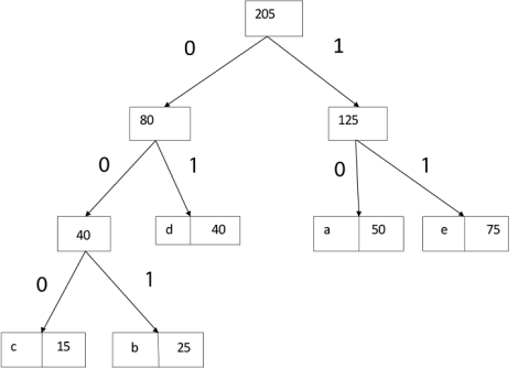
A12) Huffman invented a greedy algorithm that creates an optimal prefix code called a Huffman Code.

Fig – Greedy Algorithm for constructing a Huffman Code
The algorithm builds the tree T analogous to the optimal code in a bottom-up manner. It starts with a set of |C| leaves (C is the number of characters) and performs |C| - 1 ‘merging’ operations to create the final tree. In the Huffman algorithm ‘n’ denotes the quantity of a set of characters, z indicates the parent node, and x & y are the left & right child of z respectively.
Huffman I
1. n=|C|
2. Q ← C
3. for i=1 to n-1
4. do
5. z= allocate-Node ()
6. x= left[z]=Extract-Min(Q)
7. y= right[z] =Extract-Min(Q)
8. f [z]=f[x]+f[y]
9. Insert (Q, z)
10. return Extract-Min (Q)
Example: Find an optimal Huffman Code for the following set of frequencies:
Solution:
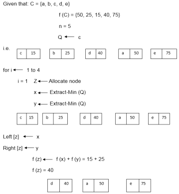
i.e.
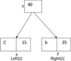
Again, for i=2
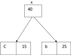
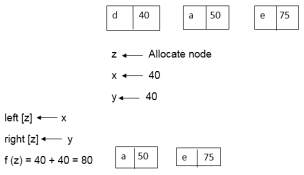
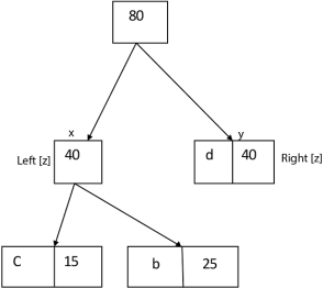
Similarly, we apply the same process we get
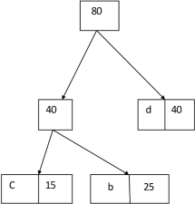
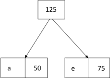
Thus, the final output is:
Q13) How we solve the Fractional knapsack problem by greedy strategy?
A13) Fractional knapsack problem can be solved by Greedy Strategy whereas 0 /1 problem is not.
In this item cannot be broken which means thief should take the item as a whole or should leave it. That’s why it is called 0/1 knapsack Problem.
Example of 0/1 Knapsack Problem:
Example: The maximum weight the knapsack can hold is W is 11. There are five items to choose from. Their weights and values are presented in the following table:

The [i, j] entry here will be V [i, j], the best value obtainable using the first “i” rows of items if the maximum capacity were j. We begin by initialization and first row.

V [i, j] = max {V [i – 1, j], vi + V [i – 1, j –wi]


The value of V [3, 7] was computed as follows:
V [3, 7] = max {V [3 – 1, 7], v3 + V [3 – 1, 7 – w3]
= max {V [2, 7], 18 + V [2, 7 – 5]}
= max {7, 18 + 6}
= 24

Finally, the output is:

The maximum value of items in the knapsack is 40, the bottom-right entry). The dynamic programming approach can now be coded as the following algorithm:
KNAPSACK (n, W)
1. for w = 0, W
2. do V [0, w] ← 0
3. for i=0, n
4. do V [i, 0] ← 0
5. for w = 0, W
6. do if (wi≤ w & vi + V [i-1, w - wi]> V [i -1, W])
7. then V [i, W] ← vi + V [i – 1, w – wi]
8. else V [i, W] ← V [i – 1, w]
Q14) Define Dynamic Programming?
A14) Dynamic programming approach is similar to divide and conquer in breaking down the problem into smaller and yet smaller possible sub-problems. But unlike, divide and conquer, these sub-problems are not solved independently. Rather, results of these smaller sub-problems are remembered and used for similar or overlapping sub-problems.
Dynamic programming approach is similar to divide and conquer in breaking down the problem into smaller and yet smaller possible sub-problems. But unlike, divide and conquer, these sub-problems are not solved independently. Rather, results of these smaller sub-problems are remembered and used for similar or overlapping sub-problems.
Dynamic programming is used where we have problems, which can be divided into similar sub-problems, so that their results can be re-used. Mostly, these algorithms are used for optimization. Before solving the in-hand sub-problem, dynamic algorithm will try to examine the results of the previously solved sub-problems. The solutions of sub-problems are combined in order to achieve the best solution.
So, we can say that –
Q15) Describe Travelling Salesman Problem? In brief.
A15) In the traveling salesman Problem, a salesman must visit n cities. We can say that salesman wishes to make a tour or Hamiltonian cycle, visiting each city exactly once and finishing at the city he starts from. There is a non-negative cost c (i, j) to travel from the city i to city j. The goal is to find a tour of minimum cost. We assume that every two cities are connected. Such problems are called Traveling-salesman problem (TSP).
We can model the cities as a complete graph of n vertices, where each vertex represents a city.
It can be shown that TSP is NPC.
If we assume the cost function c satisfies the triangle inequality, then we can use the following approximate algorithm.
Let u, v, w be any three vertices, we have

One important observation to develop an approximate solution is if we remove an edge from H*, the tour becomes a spanning tree.
Traveling-salesman Problem
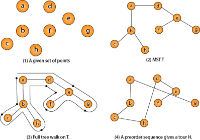
Fig - Traveling-salesman Problem
Intuitively, Approx-TSP first makes a full walk of MST T, which visits each edge exactly two times. To create a Hamiltonian cycle from the full walk, it bypasses some vertices
Q16) Define Bin packing?
A16) In case of given m elements of different weights and bins each of capacity C, assign each element to a bin so that number of total implemented bins is minimized. Assumption should be that all elements have weights less than bin capacity.
Input: weight [] = {4, 1, 8, 1, 4, 2}
Bin Capacity c = 10
Output: 2
We require at least 2 bins to accommodate all elements
First bin consists {4, 4, 2} and second bin {8, 2}
Q 17) Define Heuristics?
A17) The informed search algorithm is more useful for large search space. Informed search algorithm uses the idea of heuristic, so it is also called Heuristic search.
Heuristics function: Heuristic is a function which is used in Informed Search, and it finds the most promising path. It takes the current state of the agent as its input and produces the estimation of how close agent is from the goal. The heuristic method, however, might not always give the best solution, but it guaranteed to find a good solution in reasonable time. Heuristic function estimates how close a state is to the goal. It is represented by h(n), and it calculates the cost of an optimal path between the pair of states. The value of the heuristic function is always positive.
Admissibility of the heuristic function is given as:
h(n) <= h*(n) Here h(n) is heuristic cost, and h*(n) is the estimated cost. Hence heuristic cost should be less than or equal to the estimated cost.
Pure heuristic search is the simplest form of heuristic search algorithms. It expands nodes based on their heuristic value h(n). It maintains two lists, OPEN and CLOSED list. In the CLOSED list, it places those nodes which have already expanded and in the OPEN list, it places nodes which have yet not been expanded.
On each iteration, each node n with the lowest heuristic value is expanded and generates all its successors and n is placed to the closed list. The algorithm continues unit a goal state is found.
Q18) What is Best-first Search Algorithm?
A18) Greedy best-first search algorithm always selects the path which appears best at that moment. It is the combination of depth-first search and breadth-first search algorithms. It uses the heuristic function and search. Best-first search allows us to take the advantages of both algorithms. With the help of best-first search, at each step, we can choose the most promising node. In the best first search algorithm, we expand the node which is closest to the goal node and the closest cost is estimated by heuristic function, i.e.
Were, h(n)= estimated cost from node n to the goal.
The greedy best first algorithm is implemented by the priority queue.
Q19) What are the Advantages and Disadvantages of the best first search algorithm?
Consider the below search problem, and we will traverse it using greedy best-first search. At each iteration, each node is expanded using evaluation function f(n)=h(n), which is given in the below table.
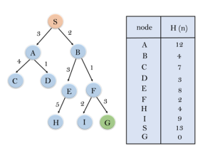
In this search example, we are using two lists which are OPEN and CLOSED Lists. Following is the iteration for traversing the above example.
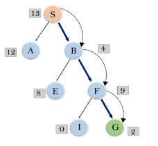
Expand the nodes of S and put in the CLOSED list
Initialization: Open [A, B], Closed [S]
Iteration 1: Open [A], Closed [S, B]
Iteration 2: Open [E, F, A], Closed [S, B]
: Open [E, A], Closed [S, B, F]
Iteration 3: Open [I, G, E, A], Closed [S, B, F]
: Open [I, E, A], Closed [S, B, F, G]
Hence the final solution path will be: S----> B----->F----> G
Time Complexity: The worst-case time complexity of Greedy best first search is O(bm).
Space Complexity: The worst-case space complexity of Greedy best first search is O(bm). Where, m is the maximum depth of the search space.
Complete: Greedy best-first search is also incomplete, even if the given state space is finite.
Optimal: Greedy best first search algorithm is not optimal.
Q20) Describe A* search algorithm?
A20) A* search is the most commonly known form of best-first search. It uses heuristic function h(n), and cost to reach the node n from the start state g(n). It has combined features of UCS and greedy best-first search, by which it solves the problem efficiently. A* search algorithm finds the shortest path through the search space using the heuristic function. This search algorithm expands less search tree and provides optimal result faster. A* algorithm is similar to UCS except that it uses g(n)+h(n) instead of g(n).
In A* search algorithm, we use search heuristic as well as the cost to reach the node. Hence, we can combine both costs as following, and this sum is called as a fitness number.

At each point in the search space, only those node is expanded which have the lowest value of f(n), and the algorithm terminates when the goal node is found.
Step1: Place the starting node in the OPEN list.
Step 2: Check if the OPEN list is empty or not, if the list is empty then return failure and stops.
Step 3: Select the node from the OPEN list which has the smallest value of evaluation function (g+h), if node n is goal node, then return success and stop, otherwise
Step 4: Expand node n and generate all of its successors, and put n into the closed list. For each successor n', check whether n' is already in the OPEN or CLOSED list, if not then compute evaluation function for n' and place into Open list.
Step 5: Else if node n' is already in OPEN and CLOSED, then it should be attached to the back pointer which reflects the lowest g(n') value.
Step 6: Return to Step 2.
Q21) What are the Advantages and Disadvantages of A* search algorithm?
A21) Advantages:
In this example, we will traverse the given graph using the A* algorithm. The heuristic value of all states is given in the below table so we will calculate the f(n) of each state using the formula f(n)= g(n) + h(n), where g(n) is the cost to reach any node from start state.
Here we will use OPEN and CLOSED list.
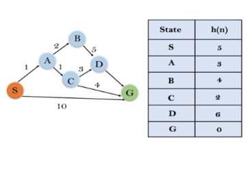
Solution:
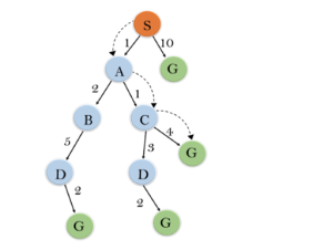
Initialization: {(S, 5)}
Iteration1: {(S--> A, 4), (S-->G, 10)}
Iteration2: {(S--> A-->C, 4), (S--> A-->B, 7), (S-->G, 10)}
Iteration3: {(S--> A-->C--->G, 6), (S--> A-->C--->D, 11), (S--> A-->B, 7), (S-->G, 10)}
Iteration 4 will give the final result, as S--->A--->C--->G it provides the optimal path with cost 6.
Points to remember:
Complete: A* algorithm is complete as long as:
Optimal: A* search algorithm is optimal if it follows below two conditions:
If the heuristic function is admissible, then A* tree search will always find the least cost path.
Time Complexity: The time complexity of A* search algorithm depends on heuristic function, and the number of nodes expanded is exponential to the depth of solution d. So, the time complexity is O(b^d), where b is the branching factor.
Space Complexity: The space complexity of A* search algorithm is O(b^d)