Unit - 2

Production, Cost and Revenue Concepts

Q1) Define production.        

A1) Since the main purpose of economic activity is to generate benefits for the individual, we count as production during a period of time all activities that either generate benefits during the period or increase the ability of society to generate benefits in the future.

Companies are important components (units) of the economic system

They are artificial units created by individuals to organize and facilitate production.

The essential characteristic of the company is that it purchases factors of production such as land, labor, capital, intermediate products and raw materials from households and other businesses and converts these resources into various goods or services that it sells to its customers. Other commercial enterprises and various government units as well as abroad.

Definition of production:

According to Bates and Parkinson:

“Production is the organized activity of converting resources into finished products in the form of goods and services. The aim of production is to meet the demand for such transformed resources”.

According to J. R. Hicks:

Production is any activity that aims to meet the needs of other people through exchange.  This definition makes it clear that in business we do not treat the mere making of things as production. What is done must be designed in such a way that it satisfies the needs.

For general purposes, it is necessary to classify production into three main groups:

1. Primary production:

Primary production is carried out by raw material industries such as agriculture and forestry, fishing, mining and oil production. Among other things, these industries are engaged in extracting the gifts of nature from the surface, below the surface and from the oceans.

2. Secondary production:

This includes production in the manufacturing industry, namely the manufacture of semi-finished and finished goods from raw materials and intermediate products - converting flour into bread or iron ore into finished steel. They are commonly referred to as the manufacturing and construction industries, such as the manufacture of automobiles, furnishings, clothing and chemicals, and engineering and construction.

3. Tertiary production:

Industries in the tertiary sector provide all the services that enable the finished goods to be placed in the hands of the consumer. In fact, these services are delivered to businesses in all industries and directly to consumers. Examples are retailers, banks, insurance companies, transportation and communications. Government services such as law, administration, education, health, and defence are also included.

Q2) Throw some light on production function.     

A2) To have clear knowledge about production and cost it’s mandatory to know the basics of production functions and understand the fundamentals in mathematical terms. We break down short-term and long-term production functions supported variable and glued factors.

What is the production function?

The functional relationship between the physical input (or factor of production) and therefore the output is named a production function. It assumed the input as an explanatory or independent variable and the output as a dependent variable.

Mathematically, you can write this as:

Q=f (L, K)

Where Q represents the output; “L” and “K” are the inputs, respectively, labour and capital (such as machinery). Note that there may be many other factors, but we are assuming a two-factor input here. Production functions are defined differently in the short term and in the long term. This distinction is crucial in microeconomics. This distinction is based on the nature of the factor input.

Inputs that change directly with the output are called variable factors. These are factors that can change. Fluctuating factors exist both in the short term and in the long term. Examples of variable factors include daily labour and raw materials.

On the other hand, factors that cannot change or change as the output changes are called fixed factors. These factors are usually characteristic only for a short or short period of time. There are no fixed factors in the long term.

Therefore, two production functions can be defined: short-term and long-term. A short-term production function defines the connection between one variable factor (keeping all other factors fixed) and therefore the output. The law of regression to factors explains such a production function.

For example, suppose that a company has 20 units of Labour and 6 acres of land, and initially uses only Labour units (variable coefficients) for that land (fixed coefficients). Thus, the ratio of land and labour is 6: 1. Now, if the company chooses to adopt 2 labour units, then the ratio of land to Labour will be 3: 1 (6: 2). Here, all factors change in the same proportion. The law used to explain this is called the law of return to scale. It measures how much of the output changes when the input changes proportionally.

Q3) Explain law of variable proportion.      

A3) The law of variable proportions or the return to factors plays an important role in the study of the theory of production. In this article, we will look at the meanings, explanations, stages, significance, and reasons behind the operation of the law of variable proportions.                                                                   

Law of variable proportions or factor of a variable

This law indicates a short-term production function in which one factor changes and the other is fixed.

Also, if you get an extra output when applying an extra unit of input, this output will be equal to or less than the output obtained from the previous unit.

The law of variable proportions relates to how the output changes when the number of units of variable factors is increased. Thus, it refers to the effect of the changing factor ratio on the output.                           

In other words, this law shows the relationship between the unit of variable factors and the volume of production in the short term. This assumes that all other factors are constant. This relationship is also known as the return to variable factors.

The law states that if we keep other factors constant, then when we increase the variable factor, the total product first increases at the rate of increase, then at the rate of decrease, and finally begins to decrease. Why is it called the law of variable proportions?

The factor ratio or factor ratio changes because one input changes and everything else remains constant. Let's take an example to better understand this:

Let's say you have 10 acres of land and 1 unit of labour for production. So, the ratio of land and labour is 10: 1. Now, if we increase the unit of Labour to 2 while keeping the land constant, then the ratio of land to Labour will be 5: 1.

Thus, as you can see, the law analyses the effect of changes in the factor ratio on the amount of out, and hence is called the law of variable proportions.

The law of proportion of variables explained

Let's understand this law with the help of another example:

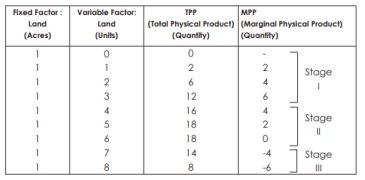
In this example, land is a fixed factor and labour is a variable factor.

The following figure describes the law of variable proportions. For a simple representation, the total physical product (TPP) curve and the limit physical product (MPP) curve are drawn as smooth curves for variable inputs (labour). Three stages of law

The law has three stages:

Stage I–TPP will increase at an increasing rate, and MPP will increase too. The MPP increases with the increase of the variable factor unit. Therefore, it's also called the stage of accelerating returns. In this example, Phase I of the law runs up to three units of labour (between points O and L).

Stage II–TPP continues to increase, but is declining. But the increase is a plus. In addition, the MPP decreases with an increase in the number of units of the variable factor. Therefore, it is called the stage of Return of decline. In this example, Stage II is performed between four to six units of labour (between points L and M). This stage reaches the point where TPP is maximum (18 in the example above) and MPP is zero (point R).

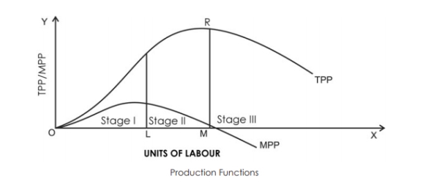
Stage III- now the TPP begins to decrease, the MPP decreases and goes to the negative. Therefore, it's called the stage of negative returns. In this example, Stage III is performed between seven and eight units of labour (from Point M onwards).

Q4) Explain law of returns to scale.       

A4) "The term scale harvest refers to changes in production when all factors change at the same rate." Koutsoyiannis

"The harvest on scale is a long-term concept, related to the behavior of total output when all inputs change." Rybavsky

There are three types of scale harvests:

1. Increasing returns on scale.

2. Harvest on a certain scale

3. Diminishing returns on scale

Explanation:

In the long run, you can increase the output by increasing all the factors at the same rate. In general, the law of harvest regarding scale refers to an increase in production due to an increase in all factors at the same rate. Such an increase is called a scale harvest.

Suppose your first production function looks like this:

P = f (L, K)

Now, if the factor of production, that is, both labor and capital, increases at the same rate, that is, x, then the product function is rewritten as:

P = f (L, K)

Now, if the factor of production, that is, both labor and capital, increases at the same rate, that is, x, then the product function is rewritten as:

1. If increases in the same proportion as the increase in factors of production i.e., , it will be constant returns to scale.

2. If increases less than proportionate increase in the factors of production i.e., , it will be diminishing returns to scale.

3. If increases more than proportionate increase in the factors of production i.e., , it will be increasing returns to scale.

Returns to scale can be shown with the help of table 8.

Table Showing different stages of return to scale

The table above describes the following three stages of harvesting in terms of scale.

1. Increasing returns on scale:

Increasing returns or reducing costs in terms of scale refers to a situation in which all factors of production increase and production increases at a higher rate. That is, when all inputs are doubled, so is the output, which increases faster than double. Therefore, it is said to be increasing returns in terms of scale. This increase is due to a number of reasons, including the sector's external economies of scale. Increasing returns in terms of scale can be explained with the help of Figure.

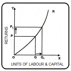
In Figure, the OX axis represents the increase in labour and capital, and the OY axis represents the increase in production. As labour and capital increase from Q to Q1, the factor of production also increases from P to P1. This is higher than the factor of production: labour and capital.

2. Diminishing returns on scale:

Diminishing returns or increased costs refer to a production situation in which production increases at a lower rate if all elements of production increase at a certain rate. That is, if the input is doubled, the output is less than doubled. An example of diminishing returns in terms of scale is when production increases by 10% after a 20% increase in labour and capital.

The main cause of diminishing returns operations in terms of scale is that the internal and external economies are less than the internal and external uneconomic. This is clear from Figure 9.

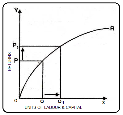
This Figure 9 shows diminishing returns in terms of scale. The OX axis gives labor and capital, and the OY axis gives output. If the factor of production increases from Q to Q1 (more quantity), but as a result the production increases, that is, P to P1 decreases. We can see that diminishing returns in terms of scale apply because the factor of production increases more and the increase in production is relatively small.

3. Harvest on a certain scale:

A harvest or a constant cost on a certain scale is a production situation in which production increases at exactly the same rate as the factor of production increases. Simply put, when the factor of production doubles, so does the production.

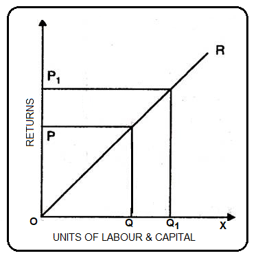
In this case, the internal and external economies are exactly the same as the internal and external economies. This situation occurs when economies of scale and economies of scale are balanced after reaching a certain production level. This is known as the homogeneous production function. The Cobb-Douglas linear homogeneous production function is a good example of this kind. This is shown in Figure 10. In Figure 10, we can see that the factor of production, that is, the increase in labor and capital, is equal to the rate of increase in the factor of production. Therefore, the result is a harvest on a certain scale.

Q5) What is total cost and fixed cost?      

A5) Total cost(TC) refers to the sum of fixed and variable costs incurred in the short term. So, the short-term cost can be expressed as follows

TC=TFC+TVC

Note that in the long run, TFC=0, so TC = TVC. So you can get the shape of the TC curve by summing the TFC curve and the TVC curve.

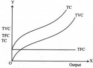
For the TC curve, the following points can be noted:

• The TC curve is shaped of reverse S. This is because of the TVC curve. Since the TFC curve is horizontal, the difference between the TC curve and the TVC curve is the same at each level of the output and is equal to the tfc. This is explained as follows: TC-TVC=TFC
• The TFC curve is parallel to the horizontal axis, and the TVC curve is inverted S-shaped.
• The law that explains the Shape of TVC and subsequent TC is called the law of variable proportions.

Fixed Cost:

1. Fixed cost (TFC)-

1. Fixed cost remains fixed in short run period. The cost does not change with the change in the level of output.
2. These costs are also called indirect costs, overhead costs, historical costs, and unavoidable costs.
3. Definition
   1. In the words of Ferguson, “Fixed cost is the sum of the ‘short run explicit fixed costs and implicit costs incurred by the entrepreneur.”

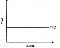
b.  From the above figure, we can see TFC curve is horizontal to X axis. TFC remains constant with proportionate change in the output.

Q6) What is total revenue? How to calculate total income?   

A6) In business and economics, one of the most important measures to assess your success and progress is to look at your gross income trends. You need to know this important metric so that you can finally calculate the total profit of your business.

Gross income in economics refers to the total income from the sale of a particular quantity of goods or services. This is the company's total revenue, calculated by multiplying the quantity of goods sold by the price of the goods. For example, if Company A creates 100 widgets and sells them for $ 50 each, the total revenue will be $ 100 * $ 50 = $ 5,000. In economics, total income is often represented as a curve in a table or graph.

It is important to note that the concept of revenue in economics usually includes two other important terms. The first term is Average Revenue (AR), which refers to the revenue per unit of output sold. This is obtained by dividing the total revenue by the number of units sold.

The second term is Marginal Revenue (MR), which is the additional revenue generated from the sale of additional units of production. In other words, it is a change in total revenue from the sale of another unit of goods. For example, if Company A sells another widget and its revenue increases from $ 5,000 to $ 5,050, the marginal revenue will be $ 50.

Determining a company's total revenue can be a useful determinant in assessing a company's financial position. The higher your total income, the more money your company is making. This is especially useful if you have a lot of money to cover. A high total income means that you have enough income to cover these costs and that you have the means to maintain ups and downs and profits for the foreseeable future.

How to calculate total income

The better you understand your total revenue, the more accurate your calculations will be. An easy way to calculate your company's total revenue is to first determine the total number of units your company has sold and the average price per unit sold. Total revenue depends on these two values. Then, to determine your total revenue, simply multiply the number of units sold by the average price per item. You also need to add interest or dividends to determine your total income.

Use the following formula when calculating your company's total revenue.

Gross income = (average price per unit sold) x (unit sales)

For service-based businesses, replace the average price per unit with the average price per service sold and the number of units sold with the number of services sold. For example:

Total revenue = (average price per service sold) x (number of services sold)

The value obtained from these calculations is total revenue. Make sure you take into account the financial changes in your company's finances, no matter how big or small.

For example, if you change the price of a unit or service sold, you should consider this change as it can distort your calculations. Also, be sure to include non-operating income such as investment income and dividend income in the calculation.

Q7) What is Average revenue?       

A7) The price that the consumer pays for the product forms the seller's income or income. The total income a seller receives from selling a certain amount of product is called gross income. If the seller sells 15 units of product at the price of Rs. Get Rs at 10 per unit. 150 from this sale, and his total income is rupees. 150.

Therefore, total revenue is obtained by multiplying the amount of production sold by the market price of the product (P.Q). On the other hand, average income is income per output. Average revenue is obtained by dividing total revenue by the number of units sold. Therefore,

Average Revenue = Total Revenue / Total Sales

AR = TR / Q

Where AR represents average revenue, TR represents total revenue, and Q represents total output produced and sold. In the above example, if the total revenue Q is equal to Rs. For selling 15 units of product, you will receive 150 and your average revenue will be equal to Rs. 150/15 = Rupee 10.Rs. 10 is the revenue earned per unit of output.

The question here is whether the average return is different from the price, or does these two concepts mean the same thing? If the seller sells different units of the product at the same price, the average revenue will be the same as the price. But if he sells different units of a particular product at different prices, the average revenue is not equal to the price.

An example clarifies this point. Suppose a seller sells two units of a product at the price of Rs. 10 per unit. The seller's total income will be rupees. It is 20, and the average return is 20/2 = Rs. 10. Therefore, the average revenue here is equal to the price of the product.

Now suppose the seller sells two units of his product and one unit to consumer A at a price of Rs. 12 and 1 unit for consumer B at price Rs. 10. His total income from the sale of two units of the product will be rupees. 22. The mean here is equal to 22/2 = Rs. 11. Therefore, in this case, if two units of the product are sold at different prices, the average revenue will not be equal to the price charged to the product.

However, in real life, you will find that the seller sells different units of the product at the same price in the market (unless the seller identifies and charges different prices for different units of the product). The average revenue is equal to the price. Therefore, economics uses average revenue and price as synonyms, except when discussing price discrimination by sellers.

The buyer's demand curve graphs the quantity requested or purchased by the buyer at different prices of the item, so it also shows the average revenue when the seller sells the different amount of item. This is because the price paid by the buyer is the revenue from the seller's point of view. Therefore, a company's average revenue curve is actually the same as the consumer demand curve.

Q8) What is marginal revenue?      

A8) Marginal revenue is the net revenue earned by selling additional units of the product. In other words, marginal revenue is added to your total revenue by selling another unit of merchandise. Algebraically, marginal revenue is added to total revenue by selling n units of product instead of n – 1. Where n is any number.

When the producer sells 10 units of product at the price Rs. 15 per unit, he gets rupees. 150 as total income. If he increases the sales of the product by 1 unit and sells 11 units, the price will drop to Rs. 14 per unit. Therefore, he will earn the total income of Rs. 154 from the sale of 11 items. This means that R has been added to the 11th output unit. 4 to total income. Therefore, Rs. 4 is the marginal revenue here.

Gross income when 10 units are sold at the price of Rs. 15 = 10 x 15 = Rs. 150

Gross income when 11 units are sold at the price of Rs. 14 = 11 x 14 = Rs 154

Marginal revenue = 154-150 = rupees. Four

The word net in the first definition of marginal revenue above is noteworthy. A complete understanding of the word "net" in the definition makes it clear why marginal revenue is not equal to price. The question is, taking the numerical example above, why is the marginal revenue from the 11th unit not equal to the price of Rs? The 11th unit was sold 14. The answer is 10 units sold at the Rs price. All prior to 15 must be sold at a discounted Rs price. 14 per unit.

This means that each of the previous 10 units has a loss of 1 rupee and the total loss of the previous 10 units due to price decline is equal to Rs. 10. The loss of revenue incurred in the previous unit is incurred as the price drops to Rs due to the sale of the additional 11th unit. 14 in all.

Therefore, to find the net amount added to the total revenue by the 11th unit, you need to deduct the revenue loss of the previous unit (Rs .10) from the price of Rs. The 11th unit is sold with others14. Therefore, the marginal revenue in this case is equal to Rs. 14 – 10 = 4. Therefore, the marginal revenue is less than the price at which additional units are sold.

From the above, it is clear that the marginal revenue can be calculated directly from the difference in total revenue before and after the sale of the additional unit, or by subtracting the loss of revenue from the previous unit due to the price decline. The price at which additional units will be sold.

Therefore, Marginal Revenue = Difference in total revenue when sales are increased from n – 1 unit to n units.

= The price of the additional unit minus the loss of revenue of the previous unit due to the price cut.

From the above, if the price drops due to additional sales, the marginal revenue will fall below the price. However, if the price remains the same when additional units are sold, as in perfect competition, the marginal revenue will be equal to the average revenue. In this case, there is no loss in the previous unit due to the price drop.

The relationship between average income and marginal income is the same as the relationship between other averages and marginal values. When the average income goes down, the marginal income becomes less than the average income. If the average income remains the same, the marginal income is equal to the average income.

Q9) State the difference between Average Revenue and Marginal Revenue.

A9) Consider the relationship between pure completion and limits, averages, and gross income under imperfect competition.

1. Under pure competition

Under pure (or complete) competition, it is assumed that there are numerous companies. Since each seller's supply is like a mighty sea drop, any increase or decrease in production by either company has no perceptible effect on aggregate supply and market prices. Only one price tends to dominate across the industry, as the collective power of supply and demand determines the price of the market. Each company must adopt a given market price and sell that quantity at the dominant market price. Simply put, the company is a "price taker" and the company's demand curve is infinitely elastic. As the company sells more and more at the specified price, its total revenue will increase, but since AR = MR, the rate of increase in total revenue will be constant.

Table: Pure Competition

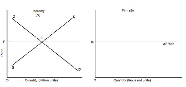
In figure 1, OX – axis represents the number of units sold and OY axis represents the price per unit. The price of the unit remains constant at P1. Consequently, AR and MR curves coincide with each other.

2.     Under imperfect competition (monopoly)

Unlike under perfect competition, companies under imperfect competition, such as under monopoly, can sell more only by lowering prices. Therefore, the average revenue curve slopes downwards, and the corresponding marginal revenue curve lies below it.

Table: Monopoly

In table, AR falls by $1 at a time whereas MR falls by $2 at each stage.

In figure, OX – axis represents the number of units of the commodity sold. OY represents the price. The AR curve as well as the MR curve slope downwards. However, the rate of all in marginal revenue is double that of the fall of the average revenue.

How much is MR below AR?

(I) When MR and AR are straight and tilted downward

If the AR and MR are straight and sloping downwards, the marginal revenue will be twice as low as the average revenue. In other words, marginal revenue cuts a line perpendicular to the y-axis in the middle of the average revenue curve. This can be proved mathematically. In Figure, AB = BC.

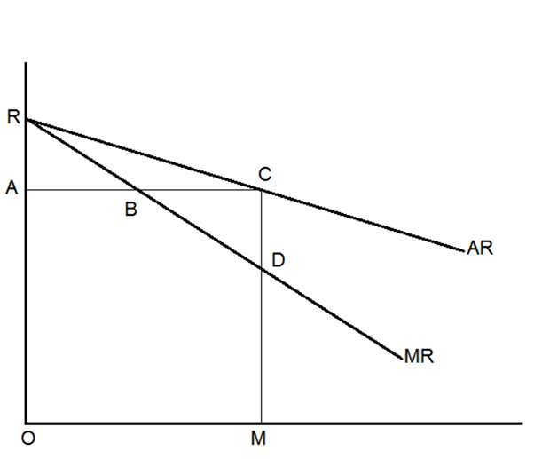
Total Revenue = Average Revenue × Output

CM × OM = Area of Rectangle ACMO

Also, Total Revenue = Area under the marginal revenue curve = RDMO

Also, ACMO = ABDMO + BCD and RDMO = ABDMO + RAB

Therefore, ABDMO + BCD = ABDMO + RAB

Or BCD = RAB

But RAB = BCD, being right angles

And RBA = CBD, being vertically opposite angles.

Thus, the two triangles are equal in area and BCD = RAB

Therefore, AB = BC

Hence, it is proved that marginal revenue curve will cut any line perpendicular to the Y-axis at halfway to the average revenue curve.

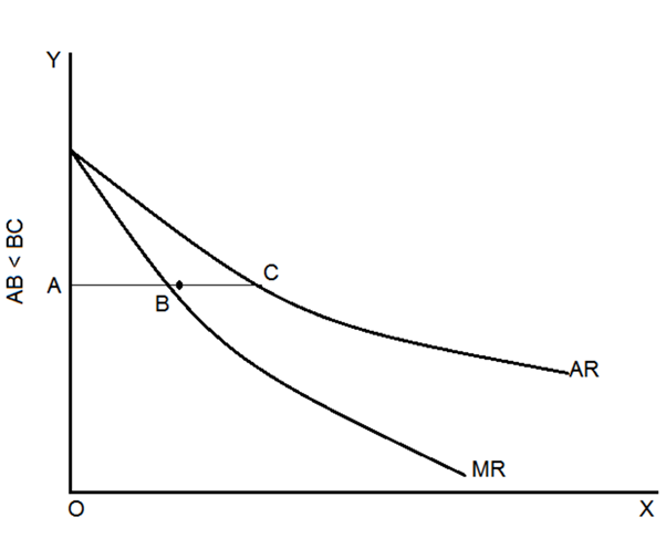
Ii) When the average profit curve is convex with respect to the origin

If the average revenue curve is convex with respect to the origin, the marginal revenue curve cuts a line perpendicular to the Y-axis at more than half of the average revenue curve. This is shown in Figure.

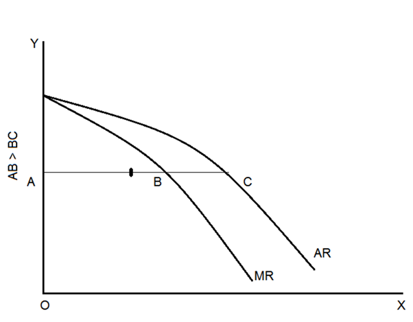
(iii) When the average profit curve is concave with respect to the origin

If the average revenue curve is concave with respect to the origin, the marginal revenue curve cuts a line that is less than half of the average revenue curve and perpendicular to the Y axis. This is shown in Figure.

Q10) Explain cost output relationship in the short run.   

A10) For research on the relationship between cost and output, 1. There are two aspects: the short-term cost-output relationship and

2. The long-term cost-output relationship.

The short term is the period during which fixed equipment (machinery, buildings, etc.) and organizational changes are not permitted. Therefore, if you need to increase production, you can do so within the limits allowed by existing fixed factors of production.

i.    Average fixed cost output:

The higher the output, the lower the fixed cost per unit, or average fixed cost. The reason is that total fixed costs remain the same and do not change with changes in production.

The relationship between output and fixed costs is universal for all types of businesses.

Therefore, average fixed costs continue to decline as production increases. The reason the total fixed costs remain the same and the average fixed costs decrease is that certain factors are inseparable. Indivisible means that if you produce less output, you cannot use that coefficient in a smaller amount. Use as a whole.

Ii.     Average variable cost and output:

As more units are produced in a particular plant, average variable costs fall first and then rise. This is because adding variable coefficient units to a fixed plant first increases the efficiency of the input and then decreases it. In fact, variable factors tend to generate somewhat more efficiently near the enterprise's optimal output than at very low levels of output.

However, when the optimum capacity is reached, the average variable cost will undoubtedly increase significantly as the output increases further. You can get more output, but the average variable cost is much higher. For example, if more and more workers are appointed. It can eventually lead to overcrowding and bad organization. In addition, workers may have to pay higher wages for overtime.

Iii.    Average total cost and output:

The average total cost, more commonly known as the average cost, decreases first and then increases. The important point to note here is that the turning point for average costs is a bit behind for average variable costs.

The average cost consists of the average fixed cost and the average variable cost. As we have seen, average fixed costs continue to decline as production increases, while average variable costs decrease first and then rise. As long as the average variable cost decreases, so does the average total cost. However, after some point, the average variable cost will rise. Here, even if the increase in variable costs is less than the decrease in fixed costs, the average total cost will continue to decrease.

Only if the increase in average variable costs is greater than the decrease in average fixed costs will the average total cost increase. Therefore, the increase in average variable costs is smaller than the decrease in average fixed costs, so the average variable costs have begun to rise, but the average total cost is still declining. The net effect is a reduction in average cost.

Minimum Cost-The output level is the level that has the lowest average total cost and is not the average variable cost. In fact, at the lowest cost output level, the average variable cost is greater than its minimum (average variable cost). The lowest cost output level is also the optimum output level. It may not be the maximum output level. Companies may decide to produce more than the lowest cost output level.

Iv.      Short-term output cost curve:

The relationship between cost and output can also be displayed using a graph. You can see that the average fixed cost curve (AFC curve) decreases as the output rises from a low level to a high level. Therefore, the shape of the average fixed cost curve is a rectangular hyperbola.

However, the average variable cost curve (AVC curve) begins to rise faster than the ATC curve. In addition, the minimum cost level of output corresponds to the point LT on the ATC curve, not the point LV on the AVC curve. Another important point is the marginal cost curve (MC curve) in Figure 3.2. It intersects both the AVC and ATC curves at the lowest point. This is very easy to explain. If the marginal cost (MC) is less than the average cost (AC), the AC will be reduced. If MC is greater than AC, raise AC. If MC is equal to AC, then AC is not raised or lowered. Therefore, the MC curve tends to intersect the AC curve at its lowest point.

Similarly, there is a view on the average variable cost curve. It makes no difference whether the MC is up or down. LT is the lowest total cost and LV is the lowest variable cost.

The interrelationships between AVC, ATC, and AFC can be summarized as follows:

1. If both AFC and AVC are reduced, so is ATC.

2. If AFC decreases but AVC increases:

(A) If the decrease in AFC is greater than the increase in AVC, the ATC will decrease.

(B) If the decrease in AFC is equal to the increase in AVC, the ATC will not decrease.

(C) If the decrease in AFC is less than the increase in AVC, the ATC will increase.

Q11) Explain cost output relationship in long run.    

A11) To study the relationship between cost and output in the long run, we need to explain the concept of long-term cost.

In the long term, it is long enough to fluctuate all costs, including those that are fixed in the short term. In the short term, output fluctuations are only possible to the extent permitted by existing fixed plants and equipment. But in the long run, the entrepreneur has many options before him, including the construction of plants of various types and sizes.

Therefore, the company has enough time to fully adapt the plant, so there are no fixed costs. And all costs fluctuate. With this in mind, long-term cost refers to the cost of producing different levels of production due to changes in plant size or production scale. The relationship between long-term cost and output is graphed by a long-term cost curve (a curve that shows how costs change when production scale changes).

The concept of long-term costs can be further explained using illustrations. Suppose a company operates under the average total cost curve U2 at a particular time and generates an OM. Here, it is desirable to generate ON. If the company continues on an older scale, its average cost curve will be NT. If the company is resized, the new cost curve will be U3. In that case, the average cost to generate an ON would be NA.

NA is less than NT. Therefore, the new scale is preferable to the old scale and should be adopted. In the long run, the average cost to generate an ON output is NA. This is sometimes referred to as the long-term cost of producing an ON output. Note that we call it NA as a long-term cost only if the U3 scale is in the planning stage and is not actually adopted. The moment you install the scale, the NA cost becomes the short-term cost to generate the ON output.

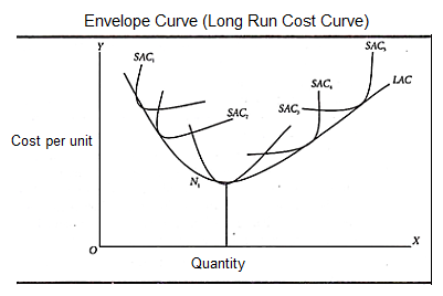
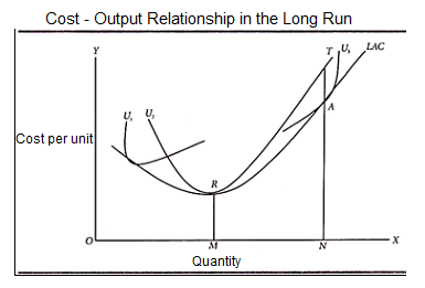
To draw a long-term cost curve, you need to start with some short-term average cost curves (SAC curves). Each such curve represents a particular scale or size of the plant, including the optimal scale. You can now draw a long-term cost curve that touches the entire family of SAC curves. That is, it touches each SAC curve at one point.

In this regard, you should be aware of the following:

1. The LAC curve touches various SAC curves. It is often referred to as the "envelope" because it is said to wrap them and the points on the SAC curve never fall below the LAC curve.

2. The LAC curve is like a U-shape or a "dish". The U-shape of the LAC curve means that the average cost will initially decrease and decrease until the optimal size of the enterprise is reached. After that, the average cost goes up continuously. That is, a plant larger than the optimal size is used.

The tendency for long-term average costs to decline as a company grows is a reflection of the cost economy as it grows, and the final rise in the long-term cost curve is primarily due to the final setting. In an uneconomical scale.

The SAC curve also has a U shape, with the difference that the LAC curve is flatter. In other words, the U-shape of the LAC curve is less noticeable. Such an economy is possible in the long run. Similarly, some of the uneconomic we face in the short term may not be faced in the long term.

3. The long-term average cost curve cannot cut the short-term average cost curve (although they are tangential to each other). This means that for a particular output, the average cost will not be higher in the long term than in the short term. This is because adjustments that reduce costs are possible in the short and long term. On the other hand, in the short term, it may not always be possible to produce a particular output in the cheapest way possible.

4. The LAC curve touches the "optimal scale" curve at the latter minimum cost point, N1.

5. The LAC curve touches the SAC curve to the left of the optimal scale curve to the left of the minimum cost point.

6. The LAC curve touches the SAC curve to the right of the optimal scale curve to the right of the minimum cost point.

Therefore, we can see that the LAC curve touches the lowest cost point for the optimal scale SAC, not for the other SAC curves.

Q12) What is Cost minimization?      

A12) Cost minimization is a basic rule used by producers to determine what mix of labor and capital produces output at the lowest cost. In other words, what the most cost-effective method of delivering goods and services would be while maintaining a desired level of quality.

An essential financial strategy it is important to understand why cost minimization is important and how it works. 

The Flexibility of the Production Function

In the long run, a producer has the flexibility over all aspects of production—how many workers to hire, how big of a factory to have, what technology to use, and so on. In more specific economic terms, a producer can vary both the amount of capital and the amount of labor it uses in the long run.

Therefore, the long-run production function has 2 inputs: capital (K) and labor (L). In the table provided here, q represents the quantity of output that is created.

Choices of Production Process

In many businesses, there are a number of ways in which a particular quantity of output can get created. If your business is making sweaters, for example, you could produce sweaters either by hiring people and buying knitting needles or by buying or renting some automated knitting machinery.

In economic terms, the first process uses a small quantity of capital and a large quantity of labor (i.e., is "labor intensive"), whereas the second process uses a large quantity of capital and a small quantity of labor (i.e., is "capital intensive"). You could even choose a process that is in between these 2 extremes.

Given that there are often a number of different ways to produce a given quantity of output, how can a company decide what mix of capital and labor to use? Not surprisingly, companies are generally going to want to choose the combination that produces a given quantity of output at the lowest cost.

Deciding the Cheapest Production

How can a company decide what combination is the cheapest?

One option would be to map out all of the combinations of labor and capital that would yield the desired quantity of output, calculate the cost of each of these options, and then choose the option with the lowest cost. Unfortunately, this can get pretty tedious and is in some cases not even feasible.

Luckily, there is a simple condition that companies can use to determine whether their mix of capital and labor is cost minimizing.

The Cost-Minimization Rule

Cost is minimized at the levels of capital and labor such that the marginal product of labor divided by the wage (w) is equal to the marginal product of capital divided by the rental price of capital (r).

More intuitively, you can think of cost being minimized and, by extension, production being most efficient when the additional output per dollar spent on each of the inputs is the same. In less formal terms, you get the same "bang for your buck" from each input. This formula can even be extended to apply to production processes that have more than 2 inputs.

To understand why this rule works, let's consider a situation that is not cost minimizing and think about why this is the case.

Let's consider a production scenario, as shown here, where the marginal product of labor divided by the wage is greater than the marginal product of capital divided by the rental price of capital.

In this situation, each dollar spent on labor creates more output than each dollar spent on capital. If you were this company, wouldn't you want to shift resources away from capital and towards labor? This would allow you to produce more output for the same cost, or, equivalently, produce the same quantity of output at a lower cost.

Of course, the concept of diminishing marginal product implies that it's generally not worthwhile to keep shifting from capital to labor forever, since increasing the quantity of labor used will decrease the marginal product of labor, and decreasing the quantity of capital used will increase the marginal product of capital. This phenomenon implies that shifting towards the input with more marginal product per dollar will eventually bring the inputs into cost-minimization balance.