Unit 3
Measures of dispersion and skewness
Question Bank
- The following table shows the sales of DVD players made by a retail store each month last year
Month | No. Of sales |
January | 25 |
Feb | 43 |
March | 39 |
April | 28 |
May | 29 |
June | 35 |
July | 32 |
August | 46 |
September | 28 |
October | 43 |
November | 51 |
December | 63 |
Solution
The range is the difference between the lowest and highest values.
The lowest number of sales = 25 in January
The highest number of sales = 63 in December
So the range = 63 - 25 = 38
2. Calculate quartile deviation from the following test scores
Sl. N o | Test scores |
1 | 17 |
2 | 17 |
3 | 26 |
4 | 27 |
5 | 30 |
6 | 30 |
7 | 31 |
8 | 37 |
Solution
First quartile (Q1)
Qi= [i * (n + 1) /4] th observation
Q1= [1 * (8 + 1) /4] th observation
Q1 = 2.25th observation
Thus, 2.25th observation lies between the 2nd and 3rd value in the ordered group, between frequency 17 and 26
First quartile (Q1) is calculated as
Q1 = 2nd observation +0.75 * (3rd observation - 2nd observation)
Q1 = 17 + 0.75 * (26 – 17) = 23.75
Third quartile (Q3)
Qi= [i * (n + 1) /4] th observation
Q3= [3 * (8 + 1) /4] th observation
Q3 = 6.75 th observation
So, 6.75 th observation lies between the 6th and 7th value in the ordered group, between frequency 30 and 31
Third quartile (Q3) is calculated as
Q3 = 6th observation +0.25 * (7th observation – 6th observation)
Q3 = 30 + 0.25 * (31 – 30) = 30.25
Now using the quartiles values Q1 and Q3, we will calculate the quartile deviation.
QD = (Q3 - Q1) / 2
QD = (30.25 – 23.75) / 2 = 3.25
3. Computation of quartile deviation for grouped test scores
Class | Frequency |
9.3-9.7 | 22 |
9.8-10.2 | 55 |
10.3-10.7 | 12 |
10.8-11.2 | 17 |
11.3-11.7 | 14 |
11.8-12.2 | 66 |
12.3-12.7 | 33 |
12.8-13.2 | 11 |
Solution
Class | Frequency | Class boundaries | CF |
9.3-9.7 | 2 | 9.25-9.75 | 2 |
9.8-10.2 | 5 | 9.75-10.25 | 2 + 5 = 7 |
10.3-10.7 | 12 | 10.25-10.75 | 7 + 12 = 19 |
10.8-11.2 | 17 | 10.75-11.25 | 19 + 17 = 36 |
11.3-11.7 | 14 | 11.25-11.75 | 36 + 14 = 50 |
11.8-12.2 | 6 | 11.75-12.25 | 50 + 6 = 56 |
12.3-12.7 | 3 | 12.25-12.75 | 56 + 3 = 59 |
12.8-13.2 | 1 | 12.75-13.25 | 59 + 1 = 60 |
First quartile (Q1)
Qi= [i * (n ) /4] th observation
Q1 = [1*(60)/4]th observation
Q1 = 15th observation
So, 15th value is in the interval 10.25-10.75
Group of Q1 = 10.25-10.75
Qi = (I + (h / f) * ( i * (N/4) – c) ; i = 1,2,3
Q1 = (10.25 + ( 0.5/ 12)* (1* (60/4) – 7)
Q1 = 10.58
Third quartile (Q3)
Qi= [i * (n) /4] th observation
Q3= [3 * (60) /4] th observation
Q3 = 45th observation
So, 45th value is in the interval 11.25-11.75
Group of Q3 = 11.25-11.75
Qi = (I + (h / f) * ( i * (N/4) – c) ; i = 1,2,3
Q3 = (11.25 + ( 0.5/ 14)* (3* (60/4) – 36)
Q3 = 11.57
QD = (Q3 - Q1) / 2
QD = (11.57 – 10.58) / 2 = 0.495
4. Calculate quartile deviation from the following data
CI | F |
10 – 15 | 6 |
15 – 20 | 10 |
20 – 25 | 15 |
25 – 30 | 22 |
30 – 40 | 12 |
40 – 50 | 9 |
50 – 60 | 4 |
60 - 70 | 2 |
Solution
CI | F | Cf |
10 – 15 | 6 | 6 |
15 – 20 | 10 | 16 |
20 – 25 | 15 | 31 |
25 – 30 | 22 | 53 |
30 – 35 | 12 | 65 |
35 – 40 | 9 | 74 |
45 – 50 | 4 | 78 |
55–60 | 2 | 80 |
First quartile (Q1)
Qi= [i * (n ) /4] th observation
Q1 = [1*(80)/4]th observation
Q1 = 20th observation
So, 20th value is in the interval 20 - 25
Group of Q1 = 20 - 25
Qi = (I + (h / f) * ( i * (N/4) – c) ; i = 1,2,3
Q1 = (20 + ( 5/ 15)* (1* (80/4) – 16)
Q1 = 21.33
Third quartile (Q3)
Qi= [i * (n) /4] th observation
Q3= [3 * (80) /4] th observation
Q3 = 60th observation
So, 60th value is in the interval 30 - 35
Group of Q3 = 30 - 35
Qi = (I + (h / f) * ( i * (N/4) – c) ; i = 1,2,3
Q3 = (30 + ( 5/ 12)* (3* (80/4) – 53)
Q3 = 32.91
QD = (Q3 - Q1) / 2
QD = (32.91 – 21.33) / 2 = 5.79
4. Computation of Mean deviation and coefficient in grouped data
Class interval | 15 – 19 | 20 – 24 | 25 – 29 | 30 – 34 | 35 – 39 | 40 – 44 | 45 - 49 |
Frequency | 1 | 4 | 6 | 9 | 5 | 3 | 2 |
Solution
Class Interval | F | X | FX | D | FD |
15 – 19 | 1 | 17 | 17 | 15 | 15 |
20 – 24 | 4 | 22 | 88 | 10 | 40 |
25 – 29 | 6 | 27 | 162 | 5 | 30 |
30 - 34 | 9 | 32 | 288 | 0 | 0 |
35 - 39 | 5 | 37 | 185 | 5 | 25 |
40 - 44 | 3 | 42 | 126 | 10 | 30 |
45 - 49 | 2 | 47 | 94 | 15 | 30 |
| N = 30 |
| ∑fx = 960 |
|  |
Mean =960/30 = 32
MD = 170 / 30 = 5.667
Coefficient of mean deviation

Coefficient of mean deviation = (5.67/32)*100 = 17.71
5. Calculate the mean deviation from continuous frequency distribution
Age group | 15 - 25 | 25 - 35 | 35 - 45 | 45 - 55 |
No. Of people | 25 | 54 | 34 | 20 |
Solution
Age group (X) | Number of people (f) | Midpoint x | Fx |
|
|
15 – 25 | 25 | 20 | 500 | 13.684 | 324.1 |
25 – 35 | 54 | 30 | 1620 | 3.684 | 198.936 |
35 – 45 | 34 | 40 | 1360 | 6.316 | 214.744 |
45 - 55 | 20 | 50 | 1000 | 16.316 | 352.32 |
| 133 |
|
|
| 1090.1 |
Mean = 4480/133 = 33.684
MD = 1090.1/133 = 8.196
6. Calculate the standard deviation using the direct method
Class interval | Frequency |
30 – 39 | 3 |
40 – 49 | 1 |
50 – 59 | 8 |
60 – 69 | 10 |
70 – 79 | 7 |
80 – 89 | 7 |
90 – 99 | 4 |
Solution
Class interval | Frequency | Mid-point x | Fx |
|
|
|
30 – 39 | 3 | 34.5 | 103.5 | -33.5 | 1122.25 | 3366.75 |
40 – 49 | 1 | 44.5 | 44.5 | -23.5 | 552.25 | 552.25 |
50 – 59 | 8 | 54.5 | 436.0 | -13.5 | 182.25 | 1458 |
60 – 69 | 10 | 64.5 | 645.0 | -3.5 | 12.25 | 122.5 |
70 – 79 | 7 | 74.5 | 521.5 | 6.5 | 42.25 | 295.75 |
80 – 89 | 7 | 84.5 | 591.5 | 16.5 | 272.25 | 1905.75 |
90 – 99 | 4 | 94.5 | 378.0 | 26.5 | 702.25 | 2809 |
| 40 |
| 2720 |
|
| 10510 |

Mean = 2720/40 = 68

SD = √10510/40 = 16.20
7. Calculate the mean and standard deviation of hours spent watching television by the 220 students.
Hours | No. Of students |
10 – 14 | 2 |
15 – 19 | 12 |
20 – 24 | 23 |
25 – 29 | 60 |
30 – 34 | 77 |
35 – 39 | 38 |
40 - 44 | 8 |
Solution
Hours | No. Of students | x | Fx |
|
|
|
10 – 14 | 2 | 12 | 24 | -17.82 | 317.49 | 634.98 |
15 – 19 | 12 | 17 | 204 | -12.82 | 164.31 | 1971.67 |
20 – 24 | 23 | 22 | 506 | -7.82 | 61.12 | 1405.85 |
25 – 29 | 60 | 27 | 1620 | -2.82 | 7.94 | 476.53 |
30 – 34 | 77 | 32 | 2464 | 2.18 | 4.76 | 366.55 |
35 – 39 | 38 | 37 | 1406 | 7.18 | 51.58 | 1959.98 |
40 - 44 | 8 | 42 | 336 | 12.18 | 148.40 | 1187.17 |
| 220 |
| 6560 |
|
| 8002.73 |

Mean = 6560/220 = 29.82

SD = √8002.73/220 = 6.03
8. Explain moments and kurtosis
Moments
Moments are a set of statistical parameters to measure a distribution. Four moments are commonly used:
• 1st moment - Mean (describes central value)
• 2nd moment - Variance (describes dispersion)
• 3rd moment - Skewness (describes asymmetry)
• 4th moment - Kurtosis (describes peakedness)
The formula for calculating moments is as follows:
1st moment = 
2nd moment =
3rd moment = 
4th moment =
Kurtosis
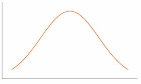
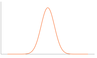
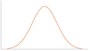
Kurtosis refers to the degree of peakedness of a frequency curve. It tells how tall and sharp the central peak is, relative to a standard bell curve of a distribution.
Excess Kurtosis
An excess kurtosis compares the kurtosis of a distribution against the kurtosis of a normal distribution. The kurtosis of a normal distribution equals 3. Therefore, the excess kurtosis is found using the formula below:
Excess Kurtosis = Kurtosis – 3
Kurtosis can be described in the following ways:
The types of kurtosis is based on the excess kurtosis of a particular distribution. The excess kurtosis can take positive or negative values, as well as values close to zero.
• Platykurtic– When the kurtosis < 0, shows a negative excess kurtosis, the frequencies throughout the curve are closer to be equal (i.e., the curve is flatter and wider)

• Leptokurtic– When the kurtosis > 0,indicates positive excess kurtosis, there are high frequencies in only a small part of the curve (i.e., the curve is more peaked)

• Mesokurtic- When the kurtosis = 0. Indicates excess kurtosis of zero or close to zero. It refers to the data flows in normal distribution.

9. Explain the difference between Skewness and Dispersion and relation among various Measures of Dispersion
Dispersion
Dispersion in statistics is a measure of how distributed the data is meaning it specifies how the values within a data set differ from one another in size. The measures of dispersion determine the spread of data around a measure of location. Measures of dispersion are range and average deviation.
Skewness
Skewness is a measure of asymmetry of distribution about a certain point. Using skewness the measure of asymmetry of a distribution is computed. On the basis of mean, median and mode skewness is measured. Depending on the data points the value of skewness can be positive, negative or undefined.
Difference between skewness and dispersion
Topic | Dispersion | Skewness |
Definition | It measures the tendency of the data set distributed over a range in statistical analysis | It measures the asymmetry in a statistical distribution from the normal distribution |
Measures | It deals with the distribution of values of a set of data around the central point | It studies whether the distribution of values is symmetric or asymmetric |
Calculation | Most common ways to calculate dispersion are range, standard deviation and average deviation | The most common ways to calculate skewness are mean, median, mode |
Variation | It determines the degree of variation in the set of data | It determines the extent of variation in terms of lower and higher values |
Application | It is used for other statistical methods such as regression analysis | It can be used for economical analysis in finance and investing |
10. Empirical relation among various Measures of Dispersion
Measures of dispersion indicate the scattering of data. It measures the disparity of data from one another.
Range - Range defines the difference between the maximum value and the minimum value given in a data set.
R = H – L
Inter quartile range - the interquartile range measures the range of the middle 50% of the values only. It is calculated as the difference between the upper and lower quartile.
Interquartile range = upper quartile – lower quartile
= Q3 – Q1
Mean deviation - The average of the absolute values of deviation from the mean, median or mode is called mean deviation
Standard deviation - standard deviation is calculated as square root of average of squared deviations taken from actual mean. It is also called root mean square deviation. This measure suffers from less drawbacks and provides accurate results.
For a symmetric distribution the relationship among Q.D., M.D. & S.D. Is:
Q. D. = 2/3 S.D.
M.D. 4/5 =S.D.
Q. D. = 5/6 M.D.
M.D. = 6/5 Q.D.
Q. D.= 2/3 S.D.
S.D. = 3/2 Q. D.
M.D. = 4/5 S.D.
S.D. = 5/4 M.D.


