Example1: Reduce the following matrix into normal form and find its rank,

Let A = 
Apply  we get
A 
Apply  we get
A 
Apply 
A 
Apply 
A 
Apply 
A 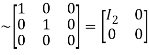
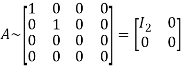
Hence the rank of matrix A is 2 i.e.  .
.
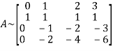
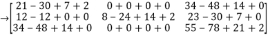
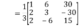
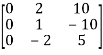
Example2: Reduce the following matrix into normal form and find its rank,

Let A = 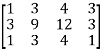
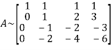
Apply  and
and 
A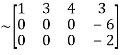
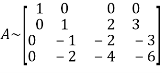
Apply 
A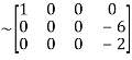
Apply 
A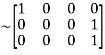
Apply 
A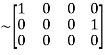
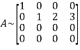
Apply 
A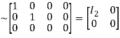
Hence the rank of the matrix A is 2 i.e.  .
.
Example3: Reduce the following matrix into normal form and find its rank,

Let A = 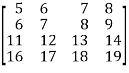
Apply 
Apply 
Apply 
Apply 
Apply  and
and 
Apply 
Hence the rank of matrix A is 2 i.e.  .
.
Example4: Reduce the following matrix to normal form of Hence find it’s rank,

Solution:
We have,


Apply 


 Rank of A = 1
Example5: Find the rank of the matrix

Solution:
We have,

Apply R12


 Rank of A = 3
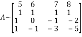
Example6: Find the rank of the following matrices by reducing it to the normal form.

Solution:

Apply C14


Example7: If  Find Two
Matrices P and Q such that PAQ is in normal form.
Solution:
Here A is a square matrix of order 3 x 3. Hence we write,
A = I3 A.I3
i.e. 


i.e. 


Example 8: Find a non – singular matrices p and Q such that P A Q is in normal form where

Solution:
Here A is a matrix of order 3 x 4. Hence we write A as,

i.e.


i.e. 


Example9: let A be a real symmetric matrix whose diagonal entries are all positive real numbers.
Is this true for all of the diagonal entries of the inverse matrix A-1 are also positive? If so, prove it. Otherwise give a counter example
Solution: The statement is false, hence we give a counter example
Let us consider the following 2 2 matrix
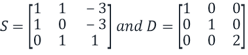
A = 
The matrix A satisfies the required conditions, that is A is symmetric and its diagonal entries are positive.
The determinant det(A) = (1)(1)-(2)(2) = -3 and the inverse of A is given by
A-1=  =
= 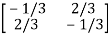
By the formula for the inverse matrix for 2 2 matrices.
This shows that the diagonal entries of the inverse matric A-1 are negative.
Skew-symmetric: A skew-symmetric matrix is a square matrix that is equal to the negative of its own transpose. Anti-symmetric matrices are commonly called as skew-symmetric matrices.
Example10: Let A and B be n n skew-matrices. Namely AT = -A and BT = -B
(a) Prove that A+B is skew-symmetric.
(b) Prove that cA is skew-symmetric for any scalar c.
(c) Let P be an m n matrix. Prove that PTAP is skew-symmetric.
Solution: (a) (A+B)T = AT + BT = (-A)+(-B) = -(A+B)
Hence A+B is skew symmetric.
(b) (cA)T = c.AT =c(-A) = -cA
Thus, cA is skew-symmetric.
(c)Let P be an m n matrix. Prove that PT AP is skew-symmetric.
Using the properties, we get,
(PT AP)T = PTAT(PT)T = PTATp
= PT (-A) P = - (PT AP)
Thus (PT AP) is skew-symmetric.
Orthogonal matrix: An orthogonal matrix is the real specialization of a unitary matrix, and thus always a normal matrix. Although we consider only real matrices here, the definition can be used for matrices with entries from any field.
Suppose A is a square matrix with real elements and of n x n order and AT is the transpose of A. Then according to the definition, if, AT = A-1 is satisfied, then,
A AT = I
Where ‘I’ is the identity matrix, A-1 is the inverse of matrix A, and ‘n’ denotes the number of rows and columns.
Example11: prove Q=  is an orthogonal matrix
Solution: Given Q = 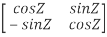
So, QT =  …..(1)
Now,we have to prove QT = Q-1
Now we find Q-1
Q-1 = 
Q-1 = 
Q-1 = 
Q-1 = 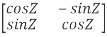 …(2)
…(2)
Now, compare (1) and (2) we get QT = Q-1
Therefore, Q is an orthogonal matrix.
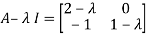
Example12: Find the eigenvalues for the following matrix?

Solution: Given 

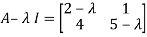

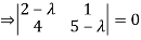
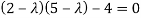
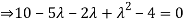
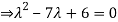
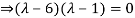
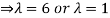
Hence the required eigenvalues are 6 and 1
Example 13: Find the eigenvalues of a 
Solution: Let A= 
Then,


These are required eigenvalues.
Example14: Let us consider the following 3 ×3 matrix
A = 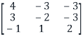
Solution: We want to diagonalize the matrix if possible.
Step 1: Find the characteristic polynomial
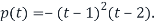
The Charcterstic polynomial p(t) of A is
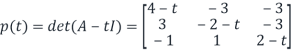
Using the cofactor expansion, we get
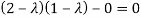
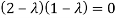
Step2: From the characteristic polynomial obtained step1, we see that eigenvalues are

And 
Step2: Find the eigenspaces
Let us first find the eigenspaces  corresponding to the eigenvalue
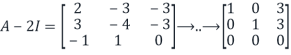
By definition,  is the null space of the matrix
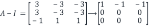
By elementary row operations.
Hence if (A-I)x=0 for x

Therefore, we have
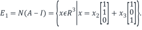
From this, we see that the set

Is a basis for the eigenvalues 
Thus, the dimension of  , which is the geometric multiplicity of
Similarly, we find a basis of the eigenspaces 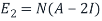 for the eigenvalue
  We have
By elementary row operations.
Then if (A-2I) x=0 for x
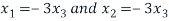
Therefore we obtain

From this we see that the set

 and the geometric multiplicity is 1.
Since for both eigenvalues, the geometric multiplicity is equal to the algebraic multiplicity, the matrix A is not defective, and hence diagonalizable.
Step4: Determine linearly independent eigenvectors
From step3, the vectors
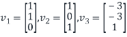
Are linearly independent eigenvectors.
Step5: Define the invertible matrix S
Define the matrix S=
S=
And the matrix S is non-singular (since the column vectors are linearly independent).
Step 6: Define the diagonal matrix D
Define the diagonal matrix
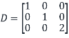
Note that (1,1) entry of D is 1 because the first column vector 
Of S is in the eigenvalues  that is
  is an eigenvector corresponding to eigenvalue
Similarly, the (2,2) entry of D is 1 because the second column  of S is in
  .
.
The (3,3)entry of D is 2 because the third column vector  of S is in
(The order you arrange the vector  to form S does not matter but once you made S, then the order of the diagonal entries is determined by S, that is , the order of eigenvectors on S)
Step7: Finish the diagonalization
Finally, we can diagonalize the matrix A as

Where
(Here you don’t have to find the inverse matrix  unless you are asked to do so).
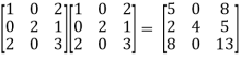
Example 15: Verify the Cayley-Hamilton theorem for A=
Solution:
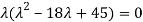
The characteristic equation of A is
P( ) =
) = =
= 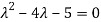


 =
= 
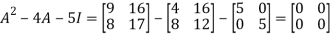
Therefore cayley-hamilton theorem is verified.
Example 16: Verify cayley-hamilton theorem for the following matrix:
A =  for
for 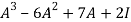
Solution:


 =
= 

 =
= 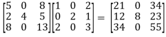

 =
= -6
-6 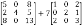 + 2
+ 2
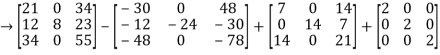
=
Hence theorem verified.
Example17: Diagonalize the matrix 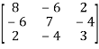
Solution: Let A = 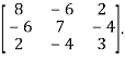
Step 1: To find the characteristic equation:
The characteristic equation of A is 
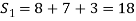
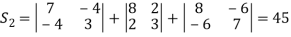
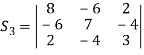
In general, 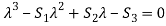 where
where


Step 2: To solve the characteristic equation.
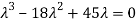
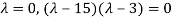

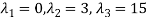 =
=
Step 3: To find the eigen vector :
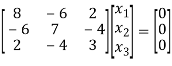
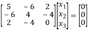
To find the eigen vector solve (A- )x=0
)x=0
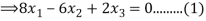
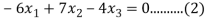
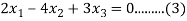
i.e. 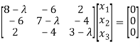
Case(i): when  , it becomes,
Solving (1) & (2) by cross-multiplication, we get
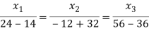
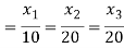
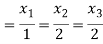
Hence the corresponding eigenvector is 
Case(ii): when  the equation (A) becomes
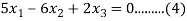
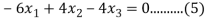
Solving (3) and (6) using cross-multiplication, we get

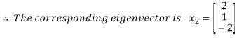
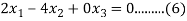
Case(iii): when  in (A)
We get the corresponding eigen vector 

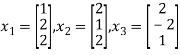
To prove these eigen vectors are orthogonal i.e. 
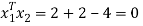
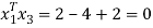
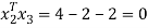
Hence the eigenvectors are orthogonal to each other
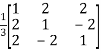
Step 4: To form the normalised matrix N
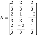
=
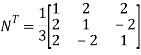
Step 5: Find 
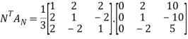
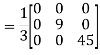
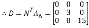
Step 6: Calculate 
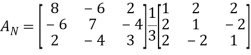
=
Step 7: Calculate