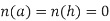
I(y)=
|
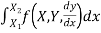
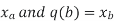
 .b) When y is a given function of xc) And is a number, when x1 and x2 have definite numerical values.
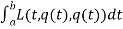
L[y(x)]=
|
S[z(x,y)] =
|
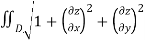
|
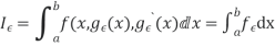
S(q) = Where, q is the function to be found: q:[a,b] t such that q is differentiable, q(a)=
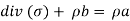
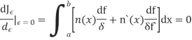
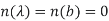
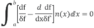
The Euler–Lagrange equation, then, is given by
Here
|


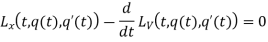


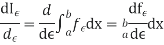
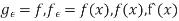
We assume that F is twice continuously differentiable A weaker assumption can be used but the proof becomes more difficult. Let Then define,
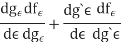
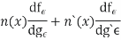
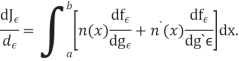
We now wish to calculate the total derivative of
It follows from the total derivation that.
So,
Where &
Using the boundary conditions
Applying the fundamental lemma of calculus of variations now yields the Euler- Lagrange eq.
|
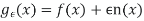


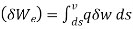
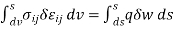
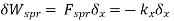
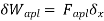
δWi= δWe Internal virtual work External virtual work
|
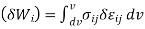
 . The imaginary displacement
  is called a virtual displacement.
 done by a force to be the equilibrium force times this small imaginary displacement
 . It should be emphasized that virtual work is not real work – no work has been performed since x is not a real displacement which has taken place; this is more like a “thought experiment”.
|
|
|

 then the virtual work is zero,
  0.
0.  is arbitrary, the system must be in equilibrium. Thus the virtual work idea gives one an alternative means of determining whether a system is in equilibrium.
  is called a variation so that, for example,
  is a variation in the displacement (from equilibrium).
|
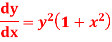
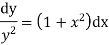
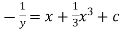
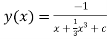
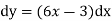
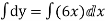
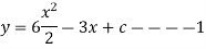
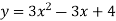
Our ODF is sepretable , thus we, seprate
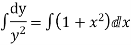
Now, integrable both sides we get,
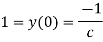
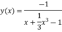
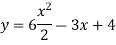
Thus , So, Applying y© =1 we obtained
Finally,
|

|

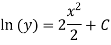
We are seprating our differential eq.
Applying y(x)=4 4=0-0+C C=4 Put this value in eq. 1
|
|

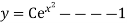
We are seperating our differential equation
Integrating both sides
Apply boundary value conditions Y(0)=3 Take exponential function both sides
C=3 Put in eq. 1
|


|
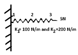
Element | K(N/m) | Nodes | Displacements m | boundary conditions |
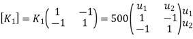
1 | 500 | 1-2 |
|
|
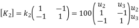
2 | 100 | 2-3 |
| ----- |


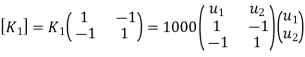
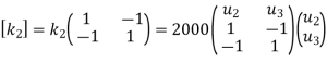
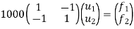
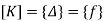
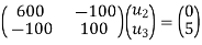
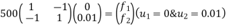
Step -2 Element stiffness matrices.
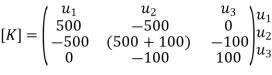
Step -3 global stiffness matrix Assemble the element stiffness matrices to get global stiffness matrix
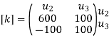
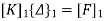
Step -4 reduced stiffness matrix imposing boundary conditions i.e Therefore, reduced stiffness matrix is.
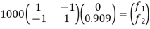
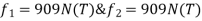
Step-5 determine unknown joint displacement Applying equation of equilibrium
Step -6 calculation of spring force. Spring -1
Spring 2 –
|


|

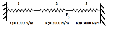
Element | K(N/m) | Nodes | Displacement | Boundary conditions | |
1 | 1000 | 1-2 |
|
| |
2 | 2000 | 2-3 |
| - | |
3 | 3000 | 3-4 |
|
| |
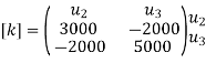
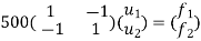
Step -2 element stiffness matrices
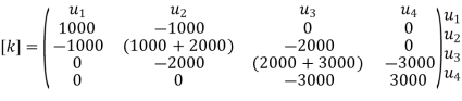
Step -3 global stiffness matrix Assemble the element stiffness matrices to get the global stiffness matrix
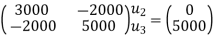
Step -4 reduced stiffness matrix Imposing boundary conditions
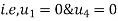
Eliminate first raw, first column & fourth raw & fourth column . Therefore reduced stiffness matrix is
Step -5 determine unknown joint displacement Applying equation of equilibrium
Step -6 calculate of spring force Spring 1 -
| |||||