Unit - 2

Introduction to Search

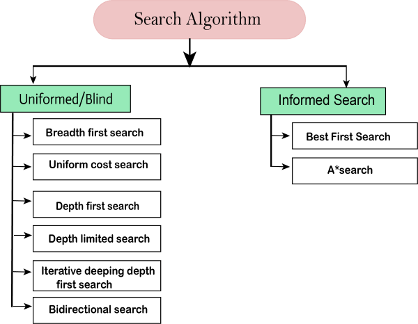
Q1) List the various search strategies.

A1)

1. BFS
2. Uniform cost search
3. DFS
4. Depth limited search
5. Iterative deepening search
6. Bidirectional search

Q2) List the various informed search strategy.

A2)

Best first search –greedy search, A* search Memory bounded search-Iterative deepening A*search -simplified memory bounded A*search -Iterative improvement search –hill climbing -simulated annealing

Q3) What is RBFS?

A3)

It keeps track of the f-value of the best alternative path available from any ancestor of the current node. RBFS remembers the f-value of the best leaf in the forgotten sub tree and therefore decide whether it’s worth re expanding the sub tree sometimes later.

Q4) List some drawbacks of hill climbing process.

A4)

Local maxima: A local maxima as opposed to a goal maximum is a peak that is lower than the highest peak in the state space. Once a local maximum is reached the algorithm will halt even though the solution may be far from satisfactory.

Plateaux: A plateaux is an area of the state space where the evaluation fn is essentially flat. The search will conduct a random walk.

Q5) What are the variants of hill climbing?

A5)

1. Stochastic hill climbing

2. First choice hill climbing

3. Simulated annealing search

4. Local beam search

5. Stochastic beam search

Q6) Give the procedure of IDA* search.

A6)

Minimize f(n)=g(n)+h(n) combines the advantage of uniform cost search + greedy search A* is complete, optimal. Its space complexity is still prohibitive.

Iterative improvement algorithms keep only a single state in memory, but can get stuck on local maxima. In this algorithm each iteration is a dfs just as in regular iterative deepening. The depth first search is modified to use an f-cost limit rather than a depth limit. Thus, each iteration expands all nodes inside the contour for the current f-cost.

Q7) List some properties of SMA* search.

A7)

1. It will utilize whatever memory is made available to it.

2. It avoids repeated states as for as its memory allow.

3. It is complete if the available memory is sufficient to store the shallowest path.

4. It is optimal if enough memory is available to store the shallowest optimal solution path.

5. Otherwise it returns the best solution that can be reached with the available memory.

6. When enough memory is available for entire search tree, the search is optimally efficient.

7. Hill climbing.

8. Simulated annealing.

Q8) Describe the Issues in knowledge representation?

A8)

Typically, a problem to solve or a task to carry out, as well as what constitutes a solution, is only given informally, such as "deliver parcels promptly when they arrive" or "fix whatever is wrong with the electrical system of the house.

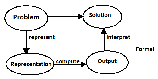
To solve a problem, the designer of a system must flesh out the task and determine what constitutes a solution; represent the problem in a language with which a computer can reason use the computer to compute an output, which is an answer presented to a user or a sequence of actions to be carried out in the environment; and interpret the output as a solution to the problem.

Knowledge is the information about a domain that can be used to solve problems in that domain. To solve many problems requires much knowledge, and this knowledge must be represented in the computer. As part of designing a program to solve problems, we must define how the knowledge will be represented. A representation scheme is the form of the knowledge that is used in an agent. A representation of some piece of knowledge is the internal representation of the knowledge.

A representation scheme specifies the form of the knowledge.

A knowledge base is the representation of all of the knowledge that is stored by an agent

Q9) Explain in details about first-order logic?

A9)

Whereas propositional logic assumes the world contains facts,

1. First-order logic (like natural language) assumes the world contains

2. Objects: people, houses, numbers, colors, baseball games, wars, …

3. Relations: red, round, prime, brother of, bigger than, part of, comes between

Atomic sentences

Atomic sentence = predicate (term1,...,termn) or term1 = term2

Term = function (term1,...,termn) or constant or variable

E.g., Brother(TaoiseachJohn,RichardTheLionheart) >

(Length(LeftLegOf(Richard)),

Length(LeftLegOf(TaoiseachJohn)))

Syntax of FOL: Basic elements

Constants TaoiseachJohn, 2, DIT…

Predicates Brother, >, …

Functions Sqrt, LeftLegOf,…

Variables x, y, a, b,…

Connectives  ¬, ⟹, ∧, ∨, ⟺

Equality =

Quantifiers ∀, ∃

Q10) Illustrate in detail about forward and backward chaining with suitable example.

A10)

Forward Chaining: The Forward chaining system, properties, algorithms, and conflict resolution strategy are illustrated.

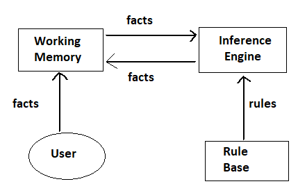
Facts are held in a working memory

1. Condition-action rules represent actions to be taken when specified facts occur in working memory.

2. Typically, actions involve adding or deleting facts from the working memory.

Properties of Forward Chaining

1. All rules which can fire do fire.

2. Can be inefficient - lead to spurious rules firing, unfocused problem

3. Solving

4. Set of rules that can fire known as conflict set.

5. Decision about which rule to fire is conflict resolution.

Forward chaining algorithm – I

Repeat

Collect the rule whose condition matches a fact in WM.

Do actions indicated by the rule. (Add facts to WM or delete facts from WM)

Until problem is solved or no condition match

Apply on the Example 2 extended (adding 2 more rules and 1 fact)

Rule R1:  IF hot AND smoky Then ADD fire

Rule R2:  IF alarm beeps  Then ADD smoky

Rule R3:  If fire   Then ADD switch_on_sprinklers

Rule R4:  If dry    Then ADD switch_on_humidifiers

Rule R5:  If sprinklers_on  Then DELETE Dry

Fact F1: alarm_beeps   [Given]

Fact  F2: hot   [Given]

Fact  F2: Dry   [Given]

Now, two rules can fire (R2 and R4)

Rule R4  ADD Humidifier is on   [from F2]

Rule R2  ADD smoky     [from F1]

[followed by  ADD fire     [from F2 by R1]

Sequence of   ADD switch_on_sprinklers  [by R3]

Actions]  DELEATE dry, ie humidifier is  [by R5]

Off a conflict!

Backward chaining

Backward chaining system and the algorithm are illustrated.

Backward chaining system

#  Backward chaining means reasoning from goals back to

Facts. The idea is to focus on the sea h.

#  Rules and facts are processed using backward chaining interpreter,

#  Checks hypothesis, e.g., "should I switch the sprinklers on?"

Backward chaining algorithm

Prove goal G

If G is in the initial facts, it is proven.

Otherwise, find a rule which can be used to conduce G, and

Try to prove each of that rule's conditions.

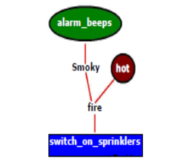
Encoding of rules

Rule R1:  IF hot AND smoky   THEN fire

Rule R2: IF alarm_beeps  THEN smoky

Rule R3: If fire    THEN switch_on_sprinklers

Q11) What does knowledge engineering in FOL MEANS?

A11)

1. Identify the task

2. Assemble the relevant knowledge

3. Decide on a vocabulary of predicates, functions, and constants

4. Encode general knowledge about the domain

5. Encode a description of the specific problem instance

6. Pose queries to the inference procedure and get answers

7. Debug the knowledge base

Q12) Explain in details about Predicate Calculus?

A12)

An interpretation over D is an assignment of the entities of D to each of the constant, variable, predicate and function symbols of a predicate calculus expression such that:

1: Each constant is assigned an element of D

2: Each variable is assigned a non-empty subset of D;(these are the allowable substitutions for

That variable)

3: Each predicate of arity n is defined on n arguments from D and defines a mapping from Dn into {T, F}

4: Each function of arity n is defined on n arguments from D and defines a mapping from Dn into D

Truth Value of Predicate Calculus expressions

• Assume an expression E and an interpretation I for E over a non-empty domain D. The truth value for E is determined by:

• The value of a constant is the element of D assigned to by I

• The value of a variable is the set of elements assigned to it by I

Similarity with Propositional logic truth values

• The value of the negation of a sentence is F if the value of the sentence is T and F otherwise

•The values for conjunction, disjunction, implication and equivalence are analogous to their propositional logic counterparts.

Q13) Explain Uniform-cost Search Algorithm?

A13)

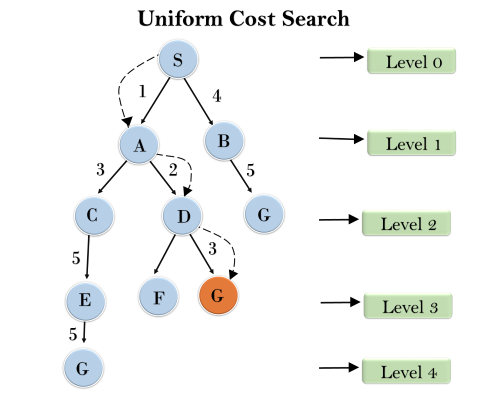
Uniform-cost search is a searching algorithm used for traversing a weighted tree or graph. This algorithm comes into play when a different cost is available for each edge. The primary goal of the uniform-cost search is to find a path to the goal node which has the lowest cumulative cost. Uniform-cost search expands nodes according to their path costs form the root node. It can be used to solve any graph/tree where the optimal cost is in demand. A uniform-cost search algorithm is implemented by the priority queue. It gives maximum priority to the lowest cumulative cost. Uniform cost search is equivalent to BFS algorithm if the path cost of all edges is the same.

Advantages:

• Uniform cost search is optimal because at every state the path with the least cost is chosen.

Disadvantages:

• It does not care about the number of steps involve in searching and only concerned about path cost. Due to which this algorithm may be stuck in an infinite loop.

Example:

Completeness:

Uniform-cost search is complete, such as if there is a solution, UCS will find it.

Time Complexity:

Let C* is Cost of the optimal solution, and ε is each step to get closer to the goal node. Then the number of steps is = C*/ε+1. Here we have taken +1, as we start from state 0 and end to C*/ε.

Hence, the worst-case time complexity of Uniform-cost search is O(b1 + [C*/ε])/.

Space Complexity:

The same logic is for space complexity so, the worst-case space complexity of Uniform-cost search is O(b1 + [C*/ε]).

Optimal:

Uniform-cost search is always optimal as it only selects a path with the lowest path cost.

Q14) Define Bidirectional Search Algorithm?

A14)

Bidirectional search algorithm runs two simultaneous searches, one form initial state called as forward-search and other from goal node called as backward-search, to find the goal node. Bidirectional search replaces one single search graph with two small subgraphs in which one starts the search from an initial vertex and other starts from goal vertex. The search stops when these two graphs intersect each other.

Bidirectional search can use search techniques such as BFS, DFS, DLS, etc.

Advantages:

• Bidirectional search is fast.
• Bidirectional search requires less memory

Disadvantages:

• Implementation of the bidirectional search tree is difficult.
• In bidirectional search, one should know the goal state in advance.

Example:

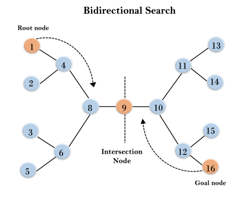
In the below search tree, bidirectional search algorithm is applied. This algorithm divides one graph/tree into two sub-graphs. It starts traversing from node 1 in the forward direction and starts from goal node 16 in the backward direction.

The algorithm terminates at node 9 where two searches meet.

Completeness: Bidirectional Search is complete if we use BFS in both searches.

Time Complexity: Time complexity of bidirectional search using BFS is O(bd).

Space Complexity: Space complexity of bidirectional search is O(bd).

Optimal: Bidirectional search is Optimal.

Q15) Define A* Search Algorithm?

A15)

A* search is the most commonly known form of best-first search. It uses heuristic function h(n), and cost to reach the node n from the start state g(n). It has combined features of UCS and greedy best-first search, by which it solves the problem efficiently. A* search algorithm finds the shortest path through the search space using the heuristic function. This search algorithm expands less search tree and provides optimal result faster. A* algorithm is similar to UCS except that it uses g(n)+h(n) instead of g(n).

In A* search algorithm, we use search heuristic as well as the cost to reach the node. Hence, we can combine both costs as following, and this sum is called as a fitness number.

At each point in the search space, only that node is expanded which have the lowest value of f(n), and the algorithm terminates when the goal node is found.

Algorithm of A* search:

Step1: Place the starting node in the OPEN list.

Step 2: Check if the OPEN list is empty or not, if the list is empty then return failure and stops.

Step 3: Select the node from the OPEN list which has the smallest value of evaluation function (g+h), if node n is goal node, then return success and stop, otherwise

Step 4: Expand node n and generate all of its successors, and put n into the closed list. For each successor n', check whether n' is already in the OPEN or CLOSED list, if not then compute evaluation function for n' and place into Open list.

Step 5: Else if node n' is already in OPEN and CLOSED, then it should be attached to the back pointer which reflects the lowest g(n') value.

Step 6: Return to Step 2. 

Advantages:

• A* search algorithm is the best algorithm than other search algorithms.
• A* search algorithm is optimal and complete.
• This algorithm can solve very complex problems.

Disadvantages:

• It does not always produce the shortest path as it mostly based on heuristics and approximation.
• A* search algorithm has some complexity issues.
• The main drawback of A* is memory requirement as it keeps all generated nodes in the memory, so it is not practical for various large-scale problems.

Example:

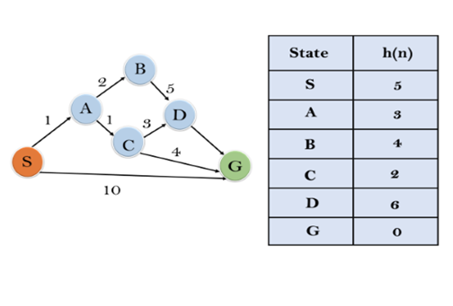
In this example, we will traverse the given graph using the A* algorithm. The heuristic value of all states is given in the below table so we will calculate the f(n) of each state using the formula f(n)= g(n) + h(n), where g(n) is the cost to reach any node from start state.

Here we will use OPEN and CLOSED list.

Solution:

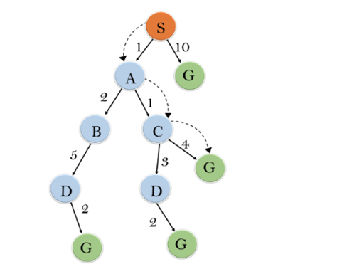
Initialization: {(S, 5)}

Iteration1: {(S--> A, 4), (S-->G, 10)}

Iteration2: {(S--> A-->C, 4), (S--> A-->B, 7), (S-->G, 10)}

Iteration3: {(S--> A-->C--->G, 6), (S--> A-->C--->D, 11), (S--> A-->B, 7), (S-->G, 10)}

Iteration 4 will give the final result, as S--->A--->C--->G it provides the optimal path with cost 6.

Points to remember:

• A* algorithm returns the path which occurred first, and it does not search for all remaining paths.
• The efficiency of A* algorithm depends on the quality of heuristic.
• A* algorithm expands all nodes which satisfy the condition f(n) <="" li="">

Complete: A* algorithm is complete as long as:

• Branching factor is finite.
• Cost at every action is fixed.

Optimal: A* search algorithm is optimal if it follows below two conditions:

• Admissible: the first condition requires for optimality is that h(n) should be an admissible heuristic for A* tree search. An admissible heuristic is optimistic in nature.
• Consistency: Second required condition is consistency for only A* graph-search.

If the heuristic function is admissible, then A* tree search will always find the least cost path.

Time Complexity: The time complexity of A* search algorithm depends on heuristic function, and the number of nodes expanded is exponential to the depth of solution d. So, the time complexity is O(b^d), where b is the branching factor.

Space Complexity: The space complexity of A* search algorithm is O(b^d)

Q16) Define MINIMAX Algorithm?

A16)

MINIMAX algorithm is a backtracking algorithm where it backtracks to pick the best move out of several choices. MINIMAX strategy follows the DFS (Depth-first search) concept. Here, we have two players MIN and MAX, and the game is played alternatively between them, i.e., when MAX made a move, then the next turn is of MIN. It means the move made by MAX is fixed and, he cannot change it. The same concept is followed in DFS strategy, i.e., we follow the same path and cannot change in the middle. That’s why in MINIMAX algorithm, instead of BFS, we follow DFS.

• Keep on generating the game tree/ search tree till a limit d.
• Compute the move using a heuristic function.
• Propagate the values from the leaf node till the current position following the minimax strategy.
• Make the best move from the choices.

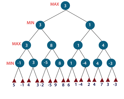
For example, in the above figure, the two players MAX and MIN are there. MAX starts the game by choosing one path and propagating all the nodes of that path. Now, MAX will backtrack to the initial node and choose the best path where his utility value will be the maximum. After this, its MIN chance. MIN will also propagate through a path and again will backtrack, but MIN will choose the path which could minimize MAX winning chances or the utility value.

So, if the level is minimizing, the node will accept the minimum value from the successor nodes. If the level is maximizing, the node will accept the maximum value from the successor.

Q17) Define Alpha - Beta pruning?

A17)

• Alpha-beta pruning is a modified version of the minimax algorithm. It is an optimization technique for the minimax algorithm.
• As we have seen in the minimax search algorithm that the number of game states it has to examine are exponential in depth of the tree. Since we cannot eliminate the exponent, but we can cut it to half. Hence there is a technique by which without checking each node of the game tree we can compute the correct minimax decision, and this technique is called pruning. This involves two threshold parameter Alpha and beta for future expansion, so it is called alpha-beta pruning. It is also called as Alpha-Beta Algorithm.
• Alpha-beta pruning can be applied at any depth of a tree, and sometimes it not only prune the tree leaves but also entire sub-tree.
• The two-parameter can be defined as:
  1. Alpha: The best (highest-value) choice we have found so far at any point along the path of Maximizer. The initial value of alpha is -∞.
  2. Beta: The best (lowest-value) choice we have found so far at any point along the path of Minimizer. The initial value of beta is +∞.
• The Alpha-beta pruning to a standard minimax algorithm returns the same move as the standard algorithm does, but it removes all the nodes which are not really affecting the final decision but making algorithm slow. Hence by pruning these nodes, it makes the algorithm fast.

Condition for Alpha-beta pruning:

The main condition which required for alpha-beta pruning is:

1. α>=β 

Key points about alpha-beta pruning:

• The Max player will only update the value of alpha.
• The Min player will only update the value of beta.
• While backtracking the tree, the node values will be passed to upper nodes instead of values of alpha and beta.
• We will only pass the alpha, beta values to the child nodes.

Pseudo-code for Alpha-beta Pruning:

1. Function minimax(node, depth, alpha, beta, maximizingPlayer) is  
2. If depth ==0 or node is a terminal node then  
3. Return static evaluation of node  
4.  
5. If MaximizingPlayer then      // for Maximizer Player  
6.   MaxEva= -infinity            
7.   For each child of node do  
8.   Eva= minimax(child, depth-1, alpha, beta, False)  
9.  MaxEva= max(maxEva, eva)   
10.  Alpha= max(alpha, maxEva)      
11.   If beta<=alpha  
12. Break  
13. Return maxEva  
14.    
15. Else                         // for Minimizer player  
16.   MinEva= +infinity   
17.   For each child of node do  
18.   Eva= minimax(child, depth-1, alpha, beta, true)  
19.   MinEva= min(minEva, eva)   
20.   Beta= min(beta, eva)  
21.    If beta<=alpha  
22.  Break          
23. Return minEva  

Working of Alpha-Beta Pruning:

Let's take an example of two-player search tree to understand the working of Alpha-beta pruning

Step 1: At the first step the, Max player will start first move from node A where α= -∞ and β= +∞, these value of alpha and beta passed down to node B where again α= -∞ and β= +∞, and Node B passes the same value to its child D.

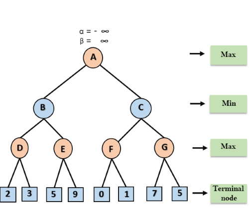
Step 2: At Node D, the value of α will be calculated as its turn for Max. The value of α is compared with firstly 2 and then 3, and the max (2, 3) = 3 will be the value of α at node D and node value will also 3.

Step 3: Now algorithm backtrack to node B, where the value of β will change as this is a turn of Min, Now β= +∞, will compare with the available subsequent nodes value, i.e. min (∞, 3) = 3, hence at node B now α= -∞, and β= 3.

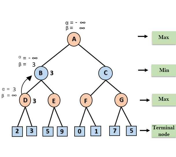
In the next step, algorithm traverse the next successor of Node B which is node E, and the values of α= -∞, and β= 3 will also be passed.

Step 4: At node E, Max will take its turn, and the value of alpha will change. The current value of alpha will be compared with 5, so max (-∞, 5) = 5, hence at node E α= 5 and β= 3, where α>=β, so the right successor of E will be pruned, and algorithm will not traverse it, and the value at node E will be 5.

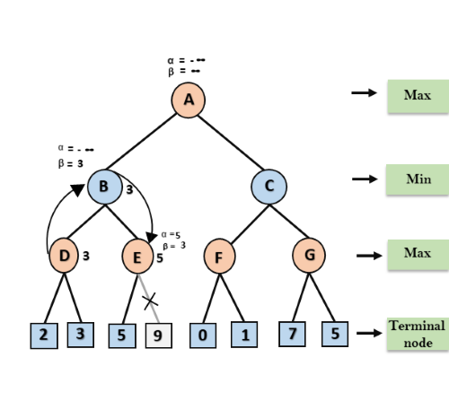
Step 5: At next step, algorithm again backtrack the tree, from node B to node A. At node A, the value of alpha will be changed the maximum available value is 3 as max (-∞, 3)= 3, and β= +∞, these two values now passes to right successor of A which is Node C.

At node C, α=3 and β= +∞, and the same values will be passed on to node F.

Step 6: At node F, again the value of α will be compared with left child which is 0, and max(3,0)= 3, and then compared with right child which is 1, and max(3,1)= 3 still α remains 3, but the node value of F will become 1.

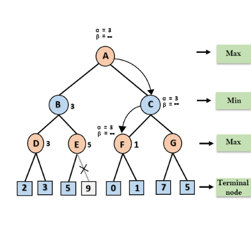
Step 7: Node F returns the node value 1 to node C, at C α= 3 and β= +∞, here the value of beta will be changed, it will compare with 1 so min (∞, 1) = 1. Now at C, α=3 and β= 1, and again it satisfies the condition α>=β, so the next child of C which is G will be pruned, and the algorithm will not compute the entire sub-tree G.

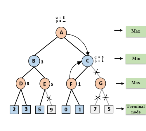
Step 8: C now returns the value of 1 to A here the best value for A is max (3, 1) = 3. Following is the final game tree which is the showing the nodes which are computed and nodes which has never computed. Hence the optimal value for the maximizer is 3 for this example.

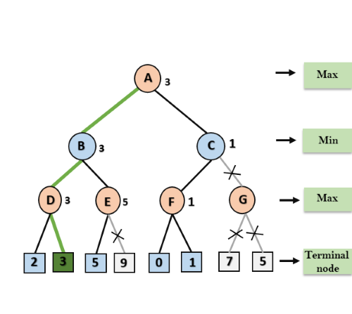
Move Ordering in Alpha-Beta pruning:

The effectiveness of alpha-beta pruning is highly dependent on the order in which each node is examined. Move order is an important aspect of alpha-beta pruning.

It can be of two types:

• Worst ordering: In some cases, alpha-beta pruning algorithm does not prune any of the leaves of the tree, and works exactly as minimax algorithm. In this case, it also consumes more time because of alpha-beta factors, such a move of pruning is called worst ordering. In this case, the best move occurs on the right side of the tree. The time complexity for such an order is O(bm).
• Ideal ordering: The ideal ordering for alpha-beta pruning occurs when lots of pruning happens in the tree, and best moves occur at the left side of the tree. We apply DFS hence it first search left of the tree and go deep twice as minimax algorithm in the same amount of time. Complexity in ideal ordering is O(bm/2).

Rules to find good ordering:

Following are some rules to find good ordering in alpha-beta pruning:

• Occur the best move from the shallowest node.
• Order the nodes in the tree such that the best nodes are checked first.
• Use domain knowledge while finding the best move. Ex: for chess, try order: captures first, then threats, then forward moves, backward moves.
• We can bookkeep the states, as there is a possibility that states may repeat.

Q18) Write the time & space complexity associated with depth limited search?

A18)

Time complexity =O (bd)

b-branching factor

d-depth of tree

Space complexity=o (bl)

Q19) List some drawbacks of hill climbing process?

A19)

Local maxima: A local maxima as opposed to a goal maximum is a peak that is lower than the highest peak in the state space. Once a local maxima is reached the algorithm will halt even though the solution may be far from satisfactory.

Plateaux: A plateaux is an area of the state space where the evaluation fn is essentially flat. The search will conduct a random walk.

Q20) Define Search Algorithm?

A20)

Search algorithms are one of the most important areas of Artificial Intelligence.

Problem-solving agents:

In Artificial Intelligence, Search techniques are universal problem-solving methods. Rational agents or Problem-solving agents in AI mostly used these search strategies or algorithms to solve a specific problem and provide the best result. Problem-solving agents are the goal-based agents and use atomic representation. In this topic, we will learn various problem-solving search algorithms.

Search Algorithm Terminologies:

• Search: Searching is a step-by-step procedure to solve a search-problem in a given search space. A search problem can have three main factors:
  1. Search Space: Search space represents a set of possible solutions, which a system may have.
  2. Start State: It is a state from where agent begins the search.
  3. Goal test: It is a function which observe the current state and returns whether the goal state is achieved or not.

Search tree: A tree representation of search problem is called Search tree. The root of the search tree is the root node which is corresponding to the initial state.

Actions: It gives the description of all the available actions to the agent.

Transition model: A description of what each action do, can be represented as a transition model.

Path Cost: It is a function which assigns a numeric cost to each path.

Solution: It is an action sequence which leads from the start node to the goal node.

Optimal Solution: If a solution has the lowest cost among all solutions.

Properties of Search Algorithms:

Following are the four essential properties of search algorithms to compare the efficiency of these algorithms:

Completeness: A search algorithm is said to be complete if it guarantees to return a solution if at least any solution exists for any random input.

Optimality: If a solution found for an algorithm is guaranteed to be the best solution (lowest path cost) among all other solutions, then such a solution for is said to be an optimal solution.

Time Complexity: Time complexity is a measure of time for an algorithm to complete its task.

Space Complexity: It is the maximum storage space required at any point during the search, as the complexity of the problem.

Types of search algorithms

Based on the search problems we can classify the search algorithms into uninformed (Blind search) search and informed search (Heuristic search) algorithms.