Unit - 5
Trees, Graphs and Combinatorics
Q1) Write short notes on a tree?
A1) An acyclic graph is one that does not have a cycle. A tree is a graph with no cycles, or an acyclic graph.
A tree, also known as a general tree, is a non-empty finite set of items called vertices or nodes that have the property of having a minimum degree of 1 and a maximum degree of n. It can be divided into n+1 disjoint subsets, with the first subset being the tree's root and the other n subsets containing the n subtree's members.
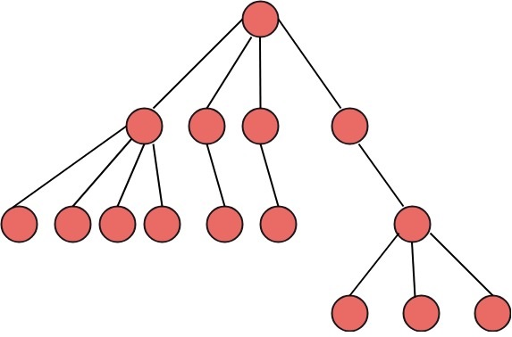
Fig: General tree
Q2) Explain binary tree?
A2) The Binary tree means that the node can have maximum two children. Here, binary name itself suggests that 'two'; therefore, each node can have either 0, 1 or 2 children.
Let's understand the binary tree through an example.

Fig - Example
The above tree is a binary tree because each node contains the utmost two children. The logical representation of the above tree is given below:
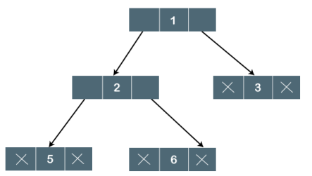
Fig - Logical representation
In the above tree, node 1 contains two pointers, i.e., left and a right pointer pointing to the left and right node respectively. The node 2 contains both the nodes (left and right node); therefore, it has two pointers (left and right). The nodes 3, 5 and 6 are the leaf nodes, so all these nodes contain NULL pointer on both left and right parts.
Properties of Binary Tree
● At each level of i, the maximum number of nodes is 2i.
● The height of the tree is defined as the longest path from the root node to the leaf node. The tree which is shown above has a height equal to 3. Therefore, the maximum number of nodes at height 3 is equal to (1+2+4+8) = 15. In general, the maximum number of nodes possible at height h is (20 + 21 + 22+….2h) = 2h+1 -1.
● The minimum number of nodes possible at height h is equal to h+1.
● If the number of nodes is minimum, then the height of the tree would be maximum. Conversely, if the number of nodes is maximum, then the height of the tree would be minimum.
If there are 'n' number of nodes in the binary tree.
Q3) Explain the type of binary tree?
A3) There are four types of Binary tree:
● Full/ proper/ strict Binary tree
● Complete Binary tree
● Perfect Binary tree
● Degenerate Binary tree
● Balanced Binary tree
- Full/ proper/ strict Binary tree
The full binary tree is also known as a strict binary tree. The tree can only be considered as the full binary tree if each node must contain either 0 or 2 children. The full binary tree can also be defined as the tree in which each node must contain 2 children except the leaf nodes.
Let's look at the simple example of the Full Binary tree.
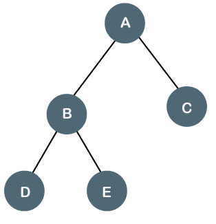
Fig - Example
In the above tree, we can observe that each node is either containing zero or two children; therefore, it is a Full Binary tree.
- Complete Binary Tree
The complete binary tree is a tree in which all the nodes are completely filled except the last level. In the last level, all the nodes must be as left as possible. In a complete binary tree, the nodes should be added from the left.
Let's create a complete binary tree.
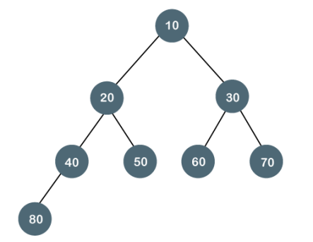
Fig - Complete binary tree
The above tree is a complete binary tree because all the nodes are completely filled, and all the nodes in the last level are added at the left first.
- Perfect Binary Tree
A tree is a perfect binary tree if all the internal nodes have 2 children, and all the leaf nodes are at the same level.
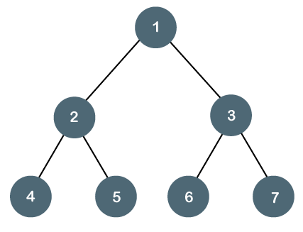
Fig - Perfect Binary Tree
Let's look at a simple example of a perfect binary tree.
The below tree is not a perfect binary tree because all the leaf nodes are not at the same level.
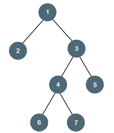
Fig - Example
Note: All the perfect binary trees are the complete binary trees as well as the full binary tree, but vice versa is not true, i.e., all complete binary trees and full binary trees are the perfect binary trees.
2. Degenerate Binary Tree
The degenerate binary tree is a tree in which all the internal nodes have only one child.
Let's understand the Degenerate binary tree through examples.
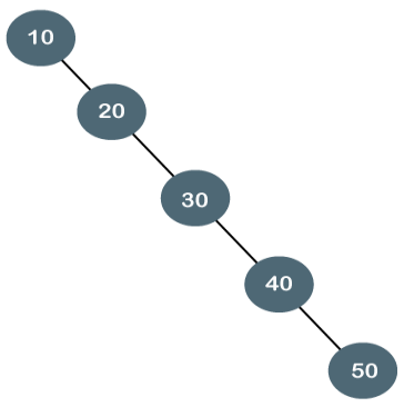
The above tree is a degenerate binary tree because all the nodes have only one child. It is also known as a right-skewed tree as all the nodes have a right child only.
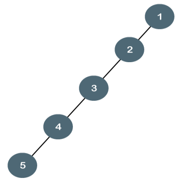
The above tree is also a degenerate binary tree because all the nodes have only one child. It is also known as a left-skewed tree as all the nodes have a left child only.
Balanced Binary Tree
The balanced binary tree is a tree in which both the left and right trees differ by at most 1. For example, AVL and Red-Black trees are balanced binary tree.
Let's understand the balanced binary tree through examples.
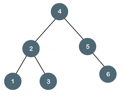
The above tree is a balanced binary tree because the difference between the left subtree and right subtree is zero.
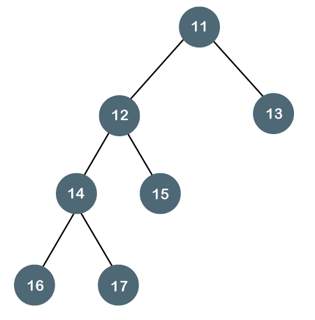
The above tree is not a balanced binary tree because the difference between the left subtree and the right subtree is greater than 1.
Q4) Explain binary tree traversal?
A4) The process of visiting the nodes is known as tree traversal. There are three types traversals used to visit a node:
● Inorder traversal
● Preorder traversal
● Postorder traversal
Tree Traversal
Traversal is a process to visit all the nodes of a tree and may print their values too. Because, all nodes are connected via edges (links) we always start from the root (head) node. That is, we cannot randomly access a node in a tree. There are three ways which we use to traverse a tree −
● In-order Traversal
● Pre-order Traversal
● Post-order Traversal
Generally, we traverse a tree to search or locate a given item or key in the tree or to print all the values it contains.
In-order Traversal
In this traversal method, the left subtree is visited first, then the root and later the right subtree. We should always remember that every node may represent a subtree itself.
If a binary tree is traversed in-order, the output will produce sorted key values in an ascending order.
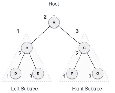
Fig - Inorder
We start from A, and following in-order traversal, we move to its left subtree B. B is also traversed in-order. The process goes on until all the nodes are visited. The output of inorder traversal of this tree will be −
D → B → E → A → F → C → G
Algorithm
Until all nodes are traversed −
Step 1 − Recursively traverse left subtree.
Step 2 − Visit root node.
Step 3 − Recursively traverse right subtree.
Pre-order Traversal
In this traversal method, the root node is visited first, then the left subtree and finally the right subtree.
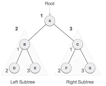
Fig – Pre order
We start from A, and following pre-order traversal, we first visit A itself and then move to its left subtree B. B is also traversed pre-order. The process goes on until all the nodes are visited. The output of pre-order traversal of this tree will be −
A → B → D → E → C → F → G
Algorithm
Until all nodes are traversed −
Step 1 − Visit root node.
Step 2 − Recursively traverse left subtree.
Step 3 − Recursively traverse right subtree.
Post-order Traversal
In this traversal method, the root node is visited last, hence the name. First, we traverse the left subtree, then the right subtree and finally the root node.
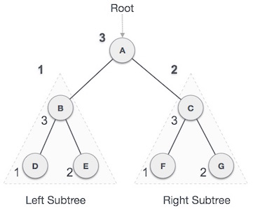
Fig – Post order
We start from A, and following post-order traversal, we first visit the left subtree B. B is also traversed post-order. The process goes on until all the nodes are visited. The output of post-order traversal of this tree will be −
D → E → B → F → G → C → A
Algorithm
Until all nodes are traversed −
Step 1 − Recursively traverse left subtree.
Step 2 − Recursively traverse right subtree.
Step 3 − Visit root node.
Q5) Explain binary search tree?
A5) Binary Tree is a special data structure used for data storage purposes. A binary tree has a special condition that each node can have a maximum of two children. A binary tree has the benefits of both an ordered array and a linked list as search is as quick as in a sorted array and insertion or deletion operation are as fast as in linked list.
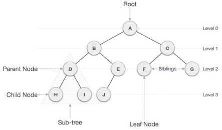
Fig - Binary Tree
Important Terms
Following are the important terms with respect to tree.
● Path − Path refers to the sequence of nodes along the edges of a tree.
● Root − The node at the top of the tree is called root. There is only one root per tree and one path from the root node to any node.
● Parent − Any node except the root node has one edge upward to a node called parent.
● Child − The node below a given node connected by its edge downward is called its child node.
● Leaf − The node which does not have any child node is called the leaf node.
● Subtree − Subtree represents the descendants of a node.
● Visiting − Visiting refers to checking the value of a node when control is on the node.
● Traversing − Traversing means passing through nodes in a specific order.
● Levels − Level of a node represents the generation of a node. If the root node is at level 0, then its next child node is at level 1, its grandchild is at level 2, and so on.
● keys − Key represents a value of a node based on which a search operation is to be carried out for a node.
Q6) Represent binary search trees?
A6) Binary Search Tree Representation
Binary Search tree exhibits a special behavior. A node's left child must have a value less than its parent's value and the node's right child must have a value greater than its parent value.
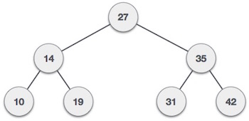
Fig - Binary Search tree
We're going to implement tree using node object and connecting them through references.
Tree Node
The code to write a tree node would be similar to what is given below. It has a data part and references to its left and right child nodes.
Struct node {
Int data;
Struct node *leftChild;
Struct node *rightChild;
};
In a tree, all nodes share a common construct.
BST Basic Operations
The basic operations that can be performed on a binary search tree data structure, are the following −
● Insert − Inserts an element in a tree/create a tree.
● Search − Searches an element in a tree.
● Preorder Traversal − Traverses a tree in a pre-order manner.
● Inorder Traversal − Traverses a tree in an in-order manner.
● Postorder Traversal − Traverses a tree in a post-order manner.
Insert Operation
Algorithm
If root is NULL
Then create root node
Return
If root exists then
Compare the data with node.data
While until insertion position is located
If data is greater than node.data
Goto right subtree
Else
Goto left subtree
End while
Insert data
End If
Implementation
The implementation of insert function should look like this −
Void insert(int data) {
Struct node *tempNode = (struct node*) malloc(sizeof(struct node));
Struct node *current;
Struct node *parent;
TempNode->data = data;
TempNode->leftChild = NULL;
TempNode->rightChild = NULL;
//if tree is empty, create root node
If(root == NULL) {
Root = tempNode;
} else {
Current = root;
Parent = NULL;
While(1) {
Parent = current;
//go to left of the tree
If(data < parent->data) {
Current = current->leftChild;
//insert to the left
If(current == NULL) {
Parent->leftChild = tempNode;
Return;
}
}
//go to right of the tree
Else {
Current = current->rightChild;
//insert to the right
If(current == NULL) {
Parent->rightChild = tempNode;
Return;
}
}
}
}
}
Search Operation
Whenever an element is to be searched, start searching from the root node, then if the data is less than the key value, search for the element in the left subtree. Otherwise, search for the element in the right subtree. Follow the same algorithm for each node.
Algorithm
If root.data is equal to search.data
Return root
Else
While data not found
If data is greater than node.data
Goto right subtree
Else
Goto left subtree
If data found
Return node
End while
Return data not found
End if
The implementation of this algorithm should look like this.
Struct node* search(int data) {
Struct node *current = root;
Printf("Visiting elements: ");
While(current->data != data) {
If(current != NULL)
Printf("%d ",current->data);
//go to left tree
If(current->data > data) {
Current = current->leftChild;
}
//else go to right tree
Else {
Current = current->rightChild;
}
//not found
If(current == NULL) {
Return NULL;
}
Return current;
}
}
Q7) Describe a graph?
A7) Graph
A graph can be defined as a group of vertices and edges that are used to connect these vertices. A graph can be seen as a cyclic tree, where the vertices (Nodes) maintain any complex relationship among them instead of having parent child relationship.
Definition
A graph G can be defined as an ordered set G(V, E) where V(G) represents the set of vertices and E(G) represents the set of edges which are used to connect these vertices.
A Graph G(V, E) with 5 vertices (A, B, C, D, E) and six edges ((A,B), (B,C), (C,E), (E,D), (D,B), (D,A)) is shown in the following figure.
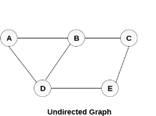
Fig – Undirected graph
Directed and Undirected Graph
A graph can be directed or undirected. However, in an undirected graph, edges are not associated with the directions with them. An undirected graph is shown in the above figure since its edges are not attached with any of the directions. If an edge exists between vertex A and B then the vertices can be traversed from B to A as well as A to B.
In a directed graph, edges form an ordered pair. Edges represent a specific path from some vertex A to another vertex B. Node A is called initial node while node B is called terminal node.
A directed graph is shown in the following figure.
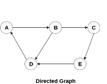
Fig – Directed graph
Graph Terminology
Path
A path can be defined as the sequence of nodes that are followed in order to reach some terminal node V from the initial node U.
Closed Path
A path will be called as closed path if the initial node is same as terminal node. A path will be closed path if V0=VN.
Simple Path
If all the nodes of the graph are distinct with an exception V0=VN, then such path P is called as closed simple path.
Cycle
A cycle can be defined as the path which has no repeated edges or vertices except the first and last vertices.
Connected Graph
A connected graph is the one in which some path exists between every two vertices (u, v) in V. There are no isolated nodes in connected graph.
Complete Graph
A complete graph is the one in which every node is connected with all other nodes. A complete graph contain n(n-1)/2 edges where n is the number of nodes in the graph.
Weighted Graph
In a weighted graph, each edge is assigned with some data such as length or weight. The weight of an edge e can be given as w(e) which must be a positive (+) value indicating the cost of traversing the edge.
Digraph
A digraph is a directed graph in which each edge of the graph is associated with some direction and the traversing can be done only in the specified direction.
Loop
An edge that is associated with the similar end points can be called as Loop.
Adjacent Nodes
If two nodes u and v are connected via an edge e, then the nodes u and v are called as neighbours or adjacent nodes.
Degree of the Node
A degree of a node is the number of edges that are connected with that node. A node with degree 0 is called as isolated node.
Q8) How to represent a graph?
A8) Graph Representation
By Graph representation, we simply mean the technique which is to be used in order to store some graph into the computer's memory.
There are two ways to store Graph into the computer's memory
1. Sequential Representation
In sequential representation, we use adjacency matrix to store the mapping represented by vertices and edges. In adjacency matrix, the rows and columns are represented by the graph vertices. A graph having n vertices, will have a dimension n x n.
An entry Mij in the adjacency matrix representation of an undirected graph G will be 1 if there exists an edge between Vi and Vj.
An undirected graph and its adjacency matrix representation is shown in the following figure.

Fig – Undirected graph and its adjacency matrix
In the above figure, we can see the mapping among the vertices (A, B, C, D, E) is represented by using the adjacency matrix which is also shown in the figure.
There exists different adjacency matrices for the directed and undirected graph. In directed graph, an entry Aij will be 1 only when there is an edge directed from Vi to Vj.
A directed graph and its adjacency matrix representation is shown in the following figure.
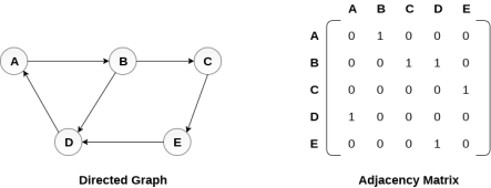
Fig - Directed graph and its adjacency matrix
Representation of weighted directed graph is different. Instead of filling the entry by 1, the Non- zero entries of the adjacency matrix are represented by the weight of respective edges.
The weighted directed graph along with the adjacency matrix representation is shown in the following figure.
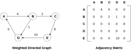
Fig - Weighted directed graph
Linked Representation
In the linked representation, an adjacency list is used to store the Graph into the computer's memory.
Consider the undirected graph shown in the following figure and check the adjacency list representation.

Fig - Undirected graph in adjacency list
An adjacency list is maintained for each node present in the graph which stores the node value and a pointer to the next adjacent node to the respective node. If all the adjacent nodes are traversed then store the NULL in the pointer field of last node of the list. The sum of the lengths of adjacency lists is equal to the twice of the number of edges present in an undirected graph.
Consider the directed graph shown in the following figure and check the adjacency list representation of the graph.
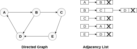
Fig - Directed graph in adjacency list
In a directed graph, the sum of lengths of all the adjacency lists is equal to the number of edges present in the graph.
In the case of weighted directed graph, each node contains an extra field that is called the weight of the node. The adjacency list representation of a directed graph is shown in the following figure.

Fig - Weighted directed graph
Q9) Define Bipartite graphs?
A9) A bipartite graph G=(V, E) has vertices V that can be partitioned into two subsets V1 and V2, with each edge of G connecting a vertex of V1 to a vertex of V2. Kmn is the symbol for it, where m and n are the vertices in V1 and V2, respectively.
Example - Draw the bipartite graphs K2, 4 and K3,4. Assume that there are any number of edges.
Solution - Draw the appropriate number of vertices on two parallel columns or rows, then connect the vertices in one column or row to the vertices in the other column or row. The bipartite graphs K2,4 and K3,4 are depicted in the figures.
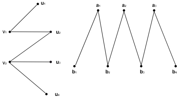
Fig: Bipartite graphs
Complete bipartite graph
If the vertices V of a graph G = (V, E) can be partitioned into two subsets V1 and V2, each vertex of V1 is connected to each vertex of V2, the graph is called a full bipartite graph. Because each of the m vertices is connected to each of the n vertices, a complete bipartite graph has m.n edges.
Example - Draw the entire bipartite graphs K3,4 and K1,5 as an example.
Solution - Draw the appropriate number of vertices in two parallel columns or rows, then connect the vertices in the first column or row to all of the vertices in the second column or row. Figure shows the graphs K3,4 and K1,5.
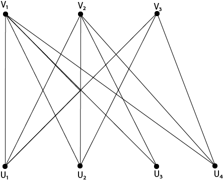
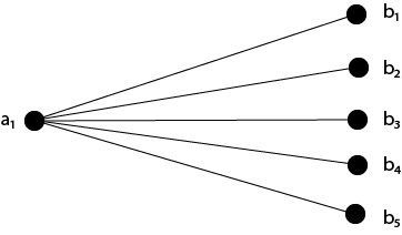
Fig: Graphs K3,4 and K1,5
Q10) Explain planner graph?
A10) "A diagram is supposed to be planar if it very well may be drawn on a plane with no edges crossing. Such a drawing is known as a planar portrayal of the graph."
A chart might be planar regardless of whether it is drawn with intersections, since it very well might be conceivable to attract it an alternate route without intersections.
For instance, consider the total chart K_{4} and its two potential planar portrayals –

Fig: Planner graph
Regions in Planar Graphs –
The planar portrayal of a diagram parts the plane into areas. These locales are limited by the edges with the exception of one district that is unbounded. For instance, think about the accompanying chart "
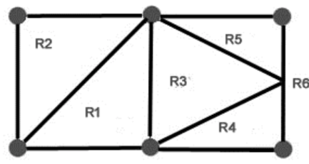
Fig: Regions planar graph
There are a sum of 6 regions with 5 limited regions and 1 unbounded area R{6}.
Q11) Explain Graph isomorphism and homeomorphism?
A11) Graph Isomorphism
Graph isomorphism is an equivalence relationship on graphs which, as such, splits the class into equivalence groups on all graphs. An isomorphism class of graphs is called a group of graphs isomorphic to one another. The two graphs shown below are isomorphic, despite their different looking drawings.

Fig: Isomorphism
Two isomorphic plots A and B and one non-isomorphic plot C; Each of them has four vertices with three corners.
Homeomorphism of graphs
If two graphs G and G* can be produced by this approach from the same graph or isomorphic graphs, they are said to be homeomorphic. The graphs (a) and (b) are not isomorphic, but they are homeomorphic since they may be created by adding appropriate vertices to the graph (c).
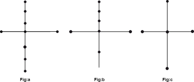
Fig: Homeomorphism graph
Properties
● If a homomorphism is a bijective mapping, it is an isomorphism.
● Homomorphism always retains a graph's edges and connectedness.
● Homomorphisms' compositions are also homomorphisms.
● It's an NP complete problem to figure out if there's any homomorphic graph of another graph.
Q12) Explain Euler and Hamiltonian paths?
A12) A Euler Path through a graph is a path whose edge list contains each edge of the graph exactly once.
Euler Circuit: A Euler Circuit is a path through a graph, in which the initial vertex appears a second time as the terminal vertex.
Euler Graph: A Euler Graph is a graph that possesses a Euler Circuit. A Euler Circuit uses every edge exactly once, but vertices may be repeated.
Example - The graph shown in fig is a Euler graph. Determine Euler Circuit for this graph.
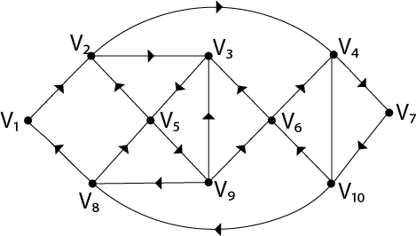
Fig: Euler graph
Solution - The Euler Circuit for this graph is
V1, V2, V3, V5, V2, V4, V7, V10, V6, V3, V9, V6, V4, V10, V8, V5, V9, V8, V1
For a connected network with no vertices of odd degrees, we can create a Euler Circuit.
State and Prove Euler's Theorem:
Consider any linked planar network with R regions, V vertices, and E edges, G= (V, E). V+R-E=2 in this case.
Proof: To prove this theorem, use induction on the number of edges.
Basis of Induction: Assume that each edge has the value e=1.
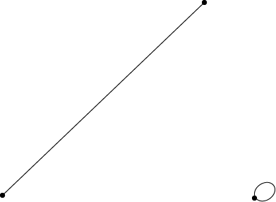
Then there are two examples, both of which have graphs in fig:
We have V=2 and R=1 in Fig. As a result, 2+1-1=2.
V=1 and R=2 are shown in Fig. As a result, 1+2-1=2.
As a result, the induction's foundation is established.
Induction step: Assume the formula is valid for connected planar graphs with K edges.
Consider the graph G, which has K+1 edges.
To begin, we assume that G is devoid of circuits. Take a vertex v and create a path that starts at v. We have a new vertex whenever we locate an edge in G since it is a circuit-free language. Finally, we'll arrive at a vertex v with degree 1. As a result, we are unable to proceed as depicted in fig.
Remove the corresponding edge incident on v and the vertex v. As a result, we have a graph G* with K edges, as shown in fig.
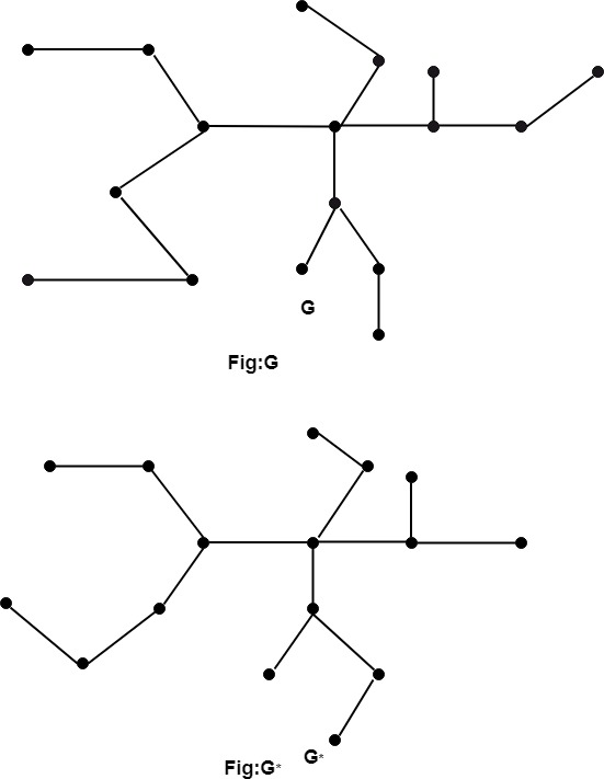
As a result, Euler's formula holds for G* by inductive assumption.
Now, G has one extra edge and one more vertex than G*, with the same number of regions. As a result, the formula also applies to G.
Second, we suppose that G contains a circuit and that e is an edge in the circuit depicted in figure:
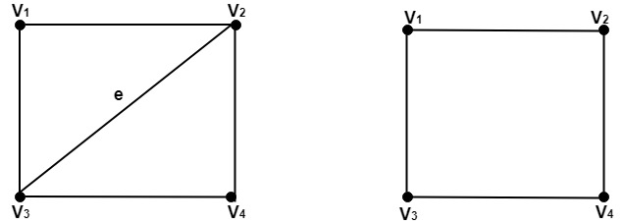
Now, because e is a portion of a two-region boundary. As a result, we merely delete the edge, leaving us with a graph G* with K edges.
As a result, Euler's formula holds for G* by inductive assumption.
G now has one more edge than G*, as well as one more area with the same number of vertices as G*. As a result, the formula also holds for G, proving the thesis by verifying the inductive steps.
Hamiltonian graph
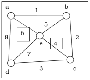
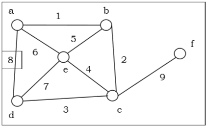
A graph that is connected If a cycle that includes every vertex of G is called a Hamiltonian cycle, then G is called a Hamiltonian graph. In graph G, a Hamiltonian walk is one that passes through each vertex precisely once.
If G is a simple graph with n vertices, where n≥3 is the number of vertices, then If each vertex v has a deg(v) ≥ n/2 value, then the graph G is a Hamiltonian graph. This is referred to as Dirac's Theorem.
G is a Hamiltonian graph if it is a simple graph with n vertices, where n≥2 is deg(x)+deg(y) ≥ n for each pair of non-adjacent vertices x and y. Ore's theorem is the name for this.
Q13) Define graph colouring?
A13) Diagram shading is the methodology of task of tones to every vertex of a chart G with the end goal that no adjoining vertices get same tone. The goal is to limit the quantity of shadings while shading a chart. The most modest number of tones needed to shading a diagram G is called its chromatic number of that chart. Diagram shading issue is a NP Complete issue.
Technique to Colour a Graph
The means needed to shading a diagram G with n number of vertices are as per the following −
Stage 1 − Arrange the vertices of the chart in some request.
Stage 2 − Choose the main vertex and shading it with the principal tone.
Stage 3 − Choose the following vertex and shading it with the most reduced numbered shading that has not been hued on any vertices neighboring it. In the event that all the contiguous vertices are hued with this tone, dole out another tone to it. Rehash this progression until all the vertices are shaded.
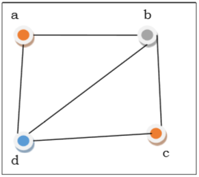
Fig: Graph colouring
In the above figure, from the start vertex an is shaded red. As the contiguous vertices of vertex an are again neighbouring, vertex b and vertex d are shaded with various tones, green and blue individually. At that point vertex c is hued however red as no adjoining vertex of c may be hued red. Consequently, we could colour the chart by 3 tones. Consequently, the chromatic number of the chart is 3.
Q14) Explain Recurrence Relation & Generating function?
A14) Recurrence Relation
The process for recursively finding the terms of a sequence is called the recurrence relation.
Definition:
A recurrence relationship is an equation that represents a series recursively where a function of the previous terms is the next term (Expressing Fn as some combination of Fi with i<n).
Example − Fibonacci series − Fn=Fn−1+Fn−2 Tower of Hanoi − Fn=2Fn−1+1
Generating function:
Generating functions are sequences in which each sequence term is expressed in a formal power series as a coefficient of a variable x.
Mathematically, the generating function would be − for an infinite number, say a0,a1,a2,...,ak,...

Some Domain Fields
For the following reasons, generating functions may be used −
● For solving a number of problems with counting. For instance, the number of ways to modify a note of Rs. 100 with denominations of Rs.1, Rs.2, Rs.5, Rs.10, Rs.20 and Rs.50 notes
● To solve relationships with recurrence
● Any of the combinatorial identities to prove
● For the finding of asymptotic formulas for sequence words
Q15) Define Recursive definition of functions?
A15) In logic and mathematics, a recursive function is a type of function or expression that predicts some concept or property of one or more variables and is defined by a procedure that generates values or instances of the function by applying a given relation or routine operation to known values of the function repeatedly.
Thoralf Albert Skolem, a pioneer in metalogic in the twentieth century, created the theory of recursive functions as a way of avoiding the so-called paradoxes of the infinite that arise in particular cases when "all" is applied to functions that span infinite classes, It accomplishes this by defining a function's range without referring to limitless classes of entities.
Taking a recognizable term like “human”—or the function “x is human”—recursion can be intuitively conveyed. “Adam and Eve are human; and any offspring of theirs is human; and any offspring of offspring... Of their offspring is human,” one can say instead of defining this notion or function by its features and dispositions.
The method known as mathematical induction is strongly related to this recursiveness in a function or notion, and it is primarily important in logic and mathematics. “x is a logical system L formula” or “x is a natural number,” for example, are typically defined recursively.
There are two pieces to a recursive definition:
- Definition of the smallest argument (usually f (0) or f (1)).
- Definition of f (n), given f (n - 1), f (n - 2), etc.
An example of a recursively defined function is as follows:


This function's values can be calculated as follows:
f (0) =5
f (1) =f (0) + 2 = 5 + 2 = 7
f (2) =f (1) + 2 = 7 + 2 = 9
f (3) =f (2) + 2 = 9 + 2 = 11
The explicitly defined function f (n) = 2n + 5 is equivalent to this recursively defined function. The recursive function, on the other hand, is only defined for nonnegative numbers.
Q16) Explain Recursive algorithms?
A16) If an algorithm solves an issue by reducing it to a smaller version of the same problem, it is called recursive.
Recursion is a type of concept and method that is crucial in both theory and practice in computer science. It is possible for recursive algorithms to be inefficient or efficient. Self-reference is a characteristic of a recursive definition or algorithm. A function is typically defined in terms of an earlier version of itself when using recursion. There must be a termination condition because this self-reference can't continue on forever. The method checks the termination condition first, and if it doesn't apply, it moves on to the self-reference.
Example: The factorial function, which is generally defined by n! = n.(n–1).(n–2).(n–3)...3.2.1 . For positive numbers and 0! = 1 for negative integers, is a classic example of a recursive definition. The following is a recursive definition of n factorial:
0! = 1
N! = N.(N!1)!; N > 0
5! = 5.4! is the formula for evaluating 5! In order to evaluate 4!, we must return to the definition, which yields 4! = 4.3! As a result, 5! = 5.4.3! Likewise, 3! = 3.2! As a result, 5! = 5.4.3.2! , 2! = 2.1! and 1! = 1.0! are the two possibilities. The first portion of the definition, however, yields 0! = 1. 5! = 5.4.3.2.1 = 120.
Now, while the preceding example may appear awkward, recursive definitions are typically easier to develop and debug in a computer environment than non-recursive definitions. The compiler is in charge of the grunt labor and record keeping. A definition similar to the two-line definition given above will be included in the program.
Q17) Write the Method of solving recurrences?
A17) Take a look at the recurrence relationship.
an = 5an-1 - 6an-2
- If the initial conditions are a0=1, a1=2, what sequence do you get? For this sequence, give a closed formula.
- If the initial conditions are a0=1, a1=3, what sequence do you get? Give a formula that is closed.
- What if a0=2, a1=5? Find a closed formula.
We've shown that recursive definitions are frequently easier to locate than closed formulas. There are a few strategies for turning recursive definitions to closed formulas, which is fortunate for us. Solving a recurrence relation is the term for this. Keep in mind that the recurrence relation is a recursive definition that does not include the initial conditions. The Fibonacci sequence, for example, has a recurrence relation of Fn = Fn-1 + Fn-2.
(This, along with the initial conditions F0 = 0, F1 = 1, completes the sequence's recursive definition.)
Example
Find the beginning conditions and a recurrence relation for 1,5,17,53, 161, 485…...
Solution
We'll attempt to solve these recurring relationships. We want to discover a function of n (a closed formula) that satisfies the recurrence relation and the initial condition, which is quite similar to solving differential equations. Finding a solution, as with differential equations, might be difficult, but verifying that the solution is accurate is simple.
Q18) What is a counting technique?
A18) Sum Rule Principle: Assume that one event E can happen in m ways and another event F can happen in n ways, and that both events cannot happen at the same time. Then E or F can happen in m + n different ways.
In general, if there are n events and no two of them occur at the same moment, the event can have n1+n2.......n different forms.
Example - If 8 male processors and 5 female processors teach DMS, the student has a total of 8+5=13 professor options.
Product Rule Principle: Assume there is an event E that can happen in m different ways, and a second event F that can happen in n different ways. Then E and F can be combined in a variety of ways.
In general, if n events occur simultaneously, they can all occur in the order represented by n1 x n2 x n3.........n ways.
Example - If there are four boys and ten girls in the class, and a boy and a girl must be picked for the class monitor, the pupils have a total of four x ten = forty options.
Mathematical Functions
Factorial Function:
Factorial n is the product of the first n natural numbers. It's represented by the letter n!, which stands for "n Factorial."
It's also possible to write Factorial n as
n! = n (n-1) (n-2) (n-3)......1.
= 1 and 0! = 1.
Q19) What is pigeonhole principle?
A19) If n+1 or more pigeons occupy n pigeonholes, then at least one pigeonhole is occupied by more than one pigeon. If n pigeonholes are occupied by kn+1 or more pigeons, where k is a positive integer, then at least one pigeonhole is inhabited by k+1 or more pigeons, according to the generalized pigeonhole principle.
Example - Find the least number of pupils in a class to ensure that three of them share the same month of birth.
Solution - Pigeonholes are defined as n = 12 months.
And k + 1 = 3
K = 2
Inclusion-Exclusion Principle:
Let A1,A2......Ar be the subset of Universal set U. Then the number m of the element which does not appear in any subset A1,A2......Ar of U.
Pigeonhole Principle
Example: Let U be the set of positive integers not exceeding 1000. Then |U|= 1000 Find |S| where S is the set of such integers which is not divisible by 3, 5 or 7?
Solution: Let A be the subset of integer which is divisible by 3
Let B be the subset of integer which is divisible by 5
Let C be the subset of integer which is divisible by 7
Then S = Ac ∩ Bc∩ Cc since each element of S is not divisible by 3, 5, or 7.
By Integer division,
|A|= 1000/3 = 333
|B|= 1000/5 = 200
|C| = 1000/7 = 142
|A∩B|=1000/15=66
|B∩C|=1000/21=47
|C∩A|=1000/35=28
|A∩B∩C|=1000/105=9
Thus, by Inclusion-Exclusion Principle
|S|=1000-(333+200+142) +(66+47+28)-9
|S|=1000-675+141-9=457