Unit 3
Statistical techniques-1
Question-1: Find the arithmetic mean of the following dataset.
Class | 0-10 | 10-20 | 20-30 | 30-40 | 40-50 |
Frequency | 7 | 8 | 20 | 10 | 5 |
Solution.
Let the assumed mean (a) = 25,
Class | Mid-value | Frequency | x – 25 = d | fd |
0-10 | 5 | 7 | -20 | -140 |
10-20 | 15 | 8 | -10 | -80 |
20-30 | 25 | 20 | 0 | 0 |
30-40 | 35 | 10 | 10 | 100 |
40-50 | 45 | 5 | 20 | 100 |
Total |
| 50 |
| -20 |

Question-2: Find the mode of the following dataset-

Solution.
Class interval | Frequency |
0 - 10 | 3 |
10 – 20 | 5 |
20 – 30 | 7 |
30 – 40 | 9 |
40 – 50 | 4 |
Here the highest frequency is 9. So that the modal class is 40-50,
Put the values in the given data-


Hence the mode is 42.86
Question-3: Define skewness and kurtosis.
Solution. Skewness-
The word skewness means lack of symmetry-
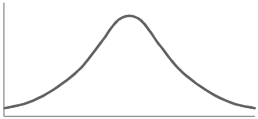
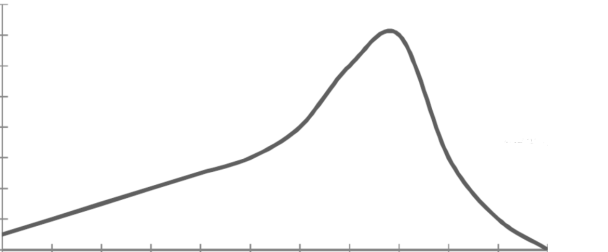
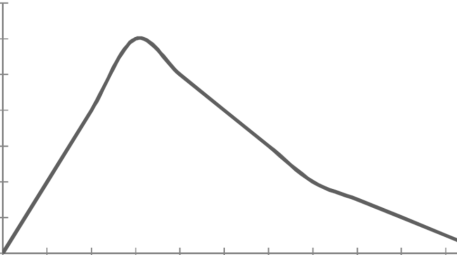
The examples of the symmetric curve, positively skewed, and negatively skewed curves are given as follows-
1. Symmetric curve-

2. Positively skewed-

3. Negatively skewed-

To measure the skewness we use Karl Pearson’s coefficient of skewness.
Then the formula is as follows-

Note- the value of Karl Pearson’s coefficient of skewness lies between -1 to +1.
Kurtosis-
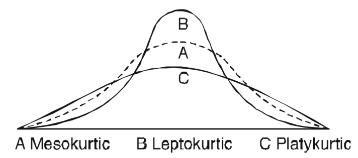
It is the measurement of the degree of peakedness of a distribution
Kurtosis is measured as-

Calculation of kurtosis-
The second and fourth central moments are used to measure kurtosis.
We use Karl Pearson’s formula to calculate kurtosis-

Now, three conditions arise-
1. If  , then the curve is mesokurtic.
2. If  , then the curve is platykurtic
3. if  , then the curve is said to be leptokurtic.
Question-4: Calculate Karl Pearson’s coefficient of skewness of marks obtained by 150 students.

Solution.
Mode is not well defined so that first we calculate mean and median-
Class | f | x | CF |
| fd |
|
0-10 | 10 | 5 | 10 | -3 | -30 | 90 |
10-20 | 40 | 15 | 50 | -2 | -80 | 160 |
20-30 | 20 | 25 | 70 | -1 | -20 | 20 |
30-40 | 0 | 35 | 70 | 0 | 0 | 0 |
40-50 | 10 | 45 | 80 | 1 | 10 | 10 |
50-60 | 40 | 55 | 120 | 2 | 80 | 160 |
60-70 | 16 | 65 | 136 | 3 | 48 | 144 |
70-80 | 14 | 75 | 150 | 4 | 56 | 244 |
Now,

And

Standard deviation-

Then-


Question-5: Calculate the median, quartiles, and the quartile coefficient of skewness from the following data:
Weight (lbs) | 70-80 | 80-90 | 90-100 | 100-110 | 110-120 | 120-130 | 130-140 | 140=150 |
No. of persons | 12 | 18 | 35 | 42 | 50 | 45 | 20 | 8 |
Solution. Here total frequency 
The cumulative frequency table is
Weight (lbs) | 70-80 | 80-90 | 90-100 | 100-110 | 110-120 | 120-130 | 130-140 | 140=150 |
Frequency | 12 | 18 | 35 | 42 | 50 | 45 | 20 | 8 |
Cumulative Frequency | 12 | 30 | 65 | 107 | 157 | 202 | 222 | 230 |
Now, N/2 =230/2= 115th item which lies in the 110 – 120 group.
Median or 
Also,  is 57.5th or 58th item which lies in the 90-100 group.

Similarly 3N/4 = 172.5 i.e.  is 173rd item which lies in the 120-130 group.

Hence quartile coefficient of skewness = 

Question-6: Find the best values of a and b so that y = a + bx fits the data given in the table
x | 0 | 1 | 2 | 3 | 4 |
y | 1.0 | 2.9 | 4.8 | 6.7 | 8.6 |
Solution.
y = a + bx
x | y | xy |
|
0 | 1.0 | 0 | 0 |
1 | 2.9 | 2.0 | 1 |
2 | 4.8 | 9.6 | 4 |
3 | 6.7 | 20.1 | 9 |
4 | 8.6 | 13.4 | 16 |
|
|
|
|
Normal equations,  y= na+ b
 x (2)
x (2)

On putting the values of 


On solving (4) and (5) we get,

On substituting the values of a and b in (1) we get

Question-7: Find the straight line that best fits the following data by using the method of least square.
X | 1 | 2 | 3 | 4 | 5 |
y | 14 | 27 | 40 | 55 | 68 |
Solution.
Suppose the straight line
y = a + bx…….. (1)
Fits the best-
Then-
x | y | xy |
|
1 | 14 | 14 | 1 |
2 | 27 | 54 | 4 |
3 | 40 | 120 | 9 |
4 | 55 | 220 | 16 |
5 | 68 | 340 | 25 |
Sum = 15 | 204 | 748 | 55 |
Normal equations are-


Put the values from the table, we get two normal equations-


On solving the above equations, we get-

So that the best fit line will be- (on putting the values of a and b in equation (1))

Questin-8: Fit the curve  by using the method of least square.
X | 1 | 2 | 3 | 4 | 5 | 6 |
Y | 7.209 | 5.265 | 3.846 | 2.809 | 2.052 | 1.499 |
Solution.
Here-


Now put-
Then we get-

x | Y |
| xY |
|
1 | 7.209 | 1.97533 | 1.97533 | 1 |
2 | 5.265 | 1.66108 | 3.32216 | 4 |
3 | 3.846 | 1.34703 | 4.04109 | 9 |
4 | 2.809 | 1.03283 | 4.13132 | 16 |
5 | 2.052 | 0.71881 | 3.59405 | 25 |
6 | 1.499 | 0.40480 | 2.4288 | 36 |
Sum = 21 |
| 7.13988 | 19.49275 | 91 |
Normal equations are-

Putting the values form the table, we get-
7.13988 = 6c + 21b
19.49275 = 21c + 91b
On solving, we get-
b = -0.3141 and c = 2.28933
c = 
Now put these values in equations (1), we get-

Questin-9: Find the correlation coefficient between the values X and Y of the dataset given below by using the short-cut method-
X | 10 | 20 | 30 | 40 | 50 |
Y | 90 | 85 | 80 | 60 | 45 |
Solution.
X | Y |
|
|
|
|
|
10 | 90 | -20 | 400 | 20 | 400 | -400 |
20 | 85 | -10 | 100 | 15 | 225 | -150 |
30 | 80 | 0 | 0 | 10 | 100 | 0 |
40 | 60 | 10 | 100 | -10 | 100 | -100 |
50 | 45 | 20 | 400 | -25 | 625 | -500 |
Sum = 150 |
360 |
0 |
1000 |
10 |
1450 |
-1150 |
Short-cut method to calculate correlation coefficient-


Question-10: The correlation table given below shows that the ages of husband and wife of 53 married couples living together on the census night of 1991. Calculate the coefficient of correlation between the age of the husband and that of the wife.
Age of husband | Age of wife | Total | ||||||
15-25 | 25-35 | 35-45 | 45-55 | 55-65 | 65-75 | |||
15-25 | 1 | 1 | - | - | - | - | 2 | |
25-35 | 2 | 12 | 1 | - | - | - | 15 | |
35-45 | - | 4 | 10 | 1 | - | - | 15 | |
45-55 | - | - | 3 | 6 | 1 | - | 10 | |
55-65 | - | - | - | 2 | 4 | 2 | 8 | |
65-75 | - | - | - | - | 1 | 2 | 3 | |
Total | 3 | 17 | 14 | 9 | 6 | 4 | 53 | |
Solution.
Age of husband | Age of wife x series | Suppose
| |||||||||||
15-25 | 25-35 | 35-45 | 45-55 | 55-65 | 65-75 |
Total f | |||||||
Years | Midpoint x | 20 | 30 | 40 | 50 | 60 | 70 | ||||||
Age group | Midpoint y |
|
| -20 | -10 | 0 | 10 | 20 | 30 |
|
|
| |
| -2 | -1 | 0 | 1 | 2 | 3 | |||||||
15-25 | 20 | -20 | -2 | 4 1 | 2 1 |
|
|
|
| 2 | -4 | 8 | 6 |
25-35 | 30 | -10 | -1 | 4 2 | 12 12 | 0 1 |
|
|
| 15 | -15 | 15 | 16 |
35-45 | 40 | 0 | 0 |
| 0 4 | 0 10 | 0 1 |
|
| 15 | 0 | 0 | 0 |
45-55 | 50 |
|
|
|
| 0 3 | 6 6 | 2 1 |
| 10 | 10 | 10 | 8 |
55-65 | 60 |
|
|
|
|
| 4 2 | 16 4 | 12 2 | 8 | 16 | 32 | 32 |
65-75 | 70 |
|
|
|
|
|
| 6 1 | 18 2 | 3 | 9 | 27 | 24 |
Total f | 3 | 17 | 14 | 9 | 6 | 4 | 53 = n | 16 | 92 | 86 | |||
| -6 | -17 | 0 | 9 | 12 | 12 | 10 | Thick figures in small sqs. for Check:
From both sides | |||||
| 12 | 17 | 0 | 9 | 24 | 36 | 98 | ||||||
| 8 | 14 | 0 | 10 | 24 | 30 | 86 | ||||||
With the help of the above correlation table, we have


Questin-11: Three judges A,B,C give the following ranks. Find which pair of judges has common approach
A | 1 | 6 | 5 | 10 | 3 | 2 | 4 | 9 | 7 | 8 |
B | 3 | 5 | 8 | 4 | 7 | 10 | 2 | 1 | 6 | 9 |
C | 6 | 4 | 9 | 8 | 1 | 2 | 3 | 10 | 5 | 7 |
Solution. Here n = 10
A (=x) | Ranks by B(=y) | C (=z) |
x-y |
y - z |
z-x |
|
|
|
1 | 3 | 6 | -2 | -3 | 5 | 4 | 9 | 25 |
6 | 5 | 4 | 1 | 1 | -2 | 1 | 1 | 4 |
5 | 8 | 9 | -3 | -1 | 4 | 9 | 1 | 16 |
10 | 4 | 8 | 6 | -4 | -2 | 36 | 16 | 4 |
3 | 7 | 1 | -4 | 6 | -2 | 16 | 36 | 4 |
2 | 10 | 2 | -8 | 8 | 0 | 64 | 64 | 0 |
4 | 2 | 3 | 2 | -1 | -1 | 4 | 1 | 1 |
9 | 1 | 10 | 8 | -9 | 1 | 64 | 81 | 1 |
7 | 6 | 5 | 1 | 1 | -2 | 1 | 1 | 4 |
8 | 9 | 7 | -1 | 2 | -1 | 1 | 4 | 1 |
Total |
|
| 0 | 0 | 0 | 200 | 214 | 60 |


Since  is maximum, the pair of judge A and C have the nearest common approach.
Question-12: Two variables X and Y are given in the dataset below, find the two lines of regression.
X | 65 | 66 | 67 | 67 | 68 | 69 | 70 | 71 |
Y | 66 | 68 | 65 | 69 | 74 | 73 | 72 | 70 |
Solution.
The two lines of regression can be expressed as-

And

x | y |
|
| xy |
65 | 66 | 4225 | 4356 | 4290 |
66 | 68 | 4356 | 4624 | 4488 |
67 | 65 | 4489 | 4225 | 4355 |
67 | 69 | 4489 | 4761 | 4623 |
68 | 74 | 4624 | 5476 | 5032 |
69 | 73 | 4761 | 5329 | 5037 |
70 | 72 | 4900 | 5184 | 5040 |
71 | 70 | 5041 | 4900 | 4970 |
Sum = 543 | 557 | 36885 | 38855 | 37835 |
Now-

And

The standard deviation of x-


Similarly-


Correlation coefficient-


Put these values in the regression line equation, we get
Regression line y on x-


Regression line x on y-


