Unit – 4

Viewing pipeline

Q1) What is the viewing pipeline?

A1) It is a term that describes a series of transformations.

The data that passed to end up image data being displayed on a device.

The viewing pipeline includes some coordinates as object coordinate, world coordinate, viewing coordinate, normalized coordinates, and device coordinates.

Object coordinate- an individual object that created by the coordinates

World coordinate- several objects into one scene

Viewing coordinate- the viewer after transformation into the coordinates system of the camera

Normalized coordinates- the projection onto a common plane that yields device-independent

Device coordinate- final mapping of normalized coordinates to a specific device

A window is a world-coordinated region that has been chosen for display. A viewport is the area on a display device to which a window is mapped. The window specifies what will be seen, while the viewport specifies where it will be presented. Rectangles in standard position, with the rectangle edges parallel to the coordinate axes, are frequently used for windows and viewports. Some applications employ other window or viewport geometries, such as general polygon shapes and circles, however these shapes take longer to analyze. A viewing transformation is the mapping of a portion of a world-coordinate scene to device coordinates in general.

The window-to-viewport transformation, often known as the windowing transformation, is a two-dimensional viewing transformation. However, watching entails more than just the transition from the window to the viewport in general. The mapping of a picture portion that falls within a rectangular window onto a defined angular viewport.

Q2) How to transform windows to viewport coordinates?

A2) We choose the window extends in viewing coordinates and selects the viewport limits in normalized coordinates once the item description has been delivered to the viewing reference frame.

The object descriptions are then converted to device coordinates that have been normalized:

We do this by employing a transformation that keeps an object's relative position in normalized space the same as it was in viewing coordinates.

If a coordinate position is in the viewing window's center:

It will appear in the viewport's center.

The mapping of the window to the viewport is shown in Figure. A point in the window at (xw, yw) is mapped to (xv, yv) in the related viewport.

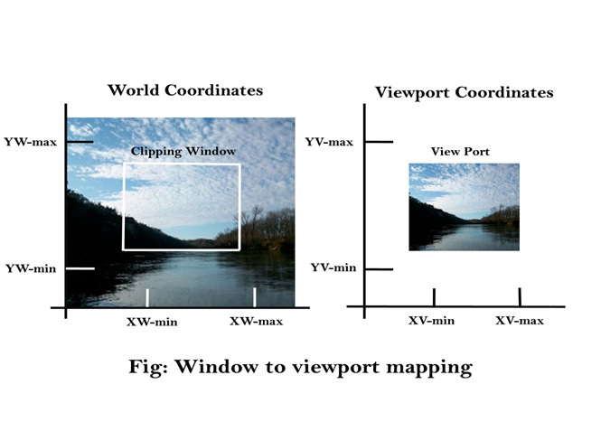
Fig 1: Window to viewport mapping

To keep the point in the viewport in the same relative position as in the window, we need to do the following:

In order to solve these impressions for the viewport position (xv, yv), we have to first solve these impressions for the viewport position (xv, yv).

Xv=xvmin+(xw-xwmin)sx

Yv=yvmin+(yw-ywmin)sy ...........equation 2

Where scaling factors are

Equations (1) and (2) can alternatively be obtained by using a set of transformations to convert the window or world coordinate area to the viewport or screen coordinate area. This dialogue is carried out using the following transformations:

●      Scale the window area to the size of the viewport with a scaling transformation using a fixed point position (xwmin,ywmin).

●      Translate the scaled window area to the viewport's position. If the scaling factors are the same (sx=sy), the relative proportions of items are maintained.

Object descriptions are mapped to the various display devices using normalized coordinates.

We can open any number of output devices in a single program, and we can perform three windows to viewport transformations for each open output device.

Workstation transformation is the name for this mapping (It is accomplished by selecting a window area in normalized space and a viewport area in the coordinates of the display device).

Workstation transformation to split a view such that different regions of normalized space can be displayed on different output devices, as seen in the figure).

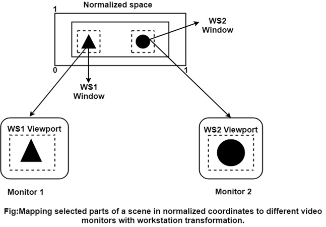
Fig 2: mapping selected parts of a scene in normalized coordinates to different video monitors with workstation transformation

Q3) What are clipping operations?

A3) A clipping algorithm, or simply clipping, is a method that detects those sections of a picture that are either inside or outside of a specific region of space. A clip window is the area against which an object will be clipped.

Clipping can be used to extract a portion of a defined scene for viewing, identify visible surfaces in three-dimensionala1 views, anti-alias line segments or object boundaries, create objects using solid-modeling procedures, display a multi window environment, and perform drawing and painting operations that allow parts of a picture to be selected for copying, moving, erasing, or duplicating. The clip window can be a general polygon or possibly have curved boundaries, depending on the application. The methods for clipping rectangular clip regions are discussed first, followed by methods for different clip-region forms. -

Only those picture parts that are within the window area should be displayed during the viewing transition (assuming that the clipping flags have not been set to noclip). Outside the window, everything is thrown away. Only the contents of the window interior are transferred to device coordinates using clipping methods in world coordinates. Alternatively, the entire world-coordinate picture can be first translated to device coordinates, or normalized device coordinates, and then cropped to viewport bounds. Clipping world coordinates removes primitives outside the window from consideration, removing the computation required to convert those primitives to device space.

By permitting the concatenation of viewing and geometric transformation matrices, viewport clipping can simplify calculations. However, viewport clipping necessitates that all objects, including those outside the window region, be transformed to device coordinates. Clipping techniques are frequently coupled with scan conversion on raster systems.

In the sections that follow, we'll look into clipping methods for the primitive types listed below.

●      Point Clipping

●      Line clipping (straight-line segments)

●      Area clipping (polygons)

●      Curve Clipping

●      Text Clipping

Q4) What do you mean by point clipping?

A4) The clipping of point from the window is very easier than line and polygon clipping.

Following figure shows the point (x,y) is given on the window representing as rectangle.

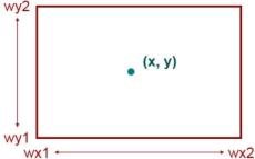
To clip a point use maximum and minimum coordinates of the window.

If X- coordinate of point lies in between Wx1 and Wx2 i.e. Wx1<= X <= Wx2 then X coordinate lies inside the window.

If Y- coordinate of point lies in between Wy1 and Wy2 i.e. Wy1<= Y <= Wy2 then Y coordinate lies inside the window.

Q5) Explain line clipping?

A5) Cohen Sutherland Method of Line Clipping

The line clipping is same as the point clipping method.

The line that is outside the window is cut and the line which is inside the window that will be displayed.

This algorithm uses the line clipping method.

The minimum coordinates for the clipping region is (XWmin, YWmin) and the maximum coordinates are (XWmax, YWmax).

As below figure 3 shows the concept of cohen Sutherland line clipping.

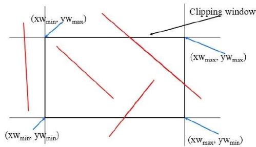
Fig. No. 3

There are three possibilities for line as-

●        The line which is completely inside the window will be accepted.

●        The line which is completely outside the window will be discarded.

●        The line which is partially inside the window in that the portion which is inside that will be shown and other part will be discarded.

The 4 bits are used to divide the entire region.

These 4 bits represent the top, bottom, top and left as the figure shows.

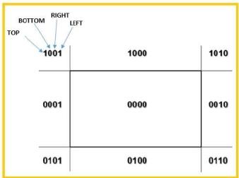
Fig. No. 4

Following are steps to perform the cohen Sutherland algorithm which are based on 4 bits that are given above.

1. Assign a region code for each endpoints.
2. If both endpoints having bits 0000 then that line will be accepted.
3. Else perform logical AND operation on the region code.
4. If the result is not 0000 then reject line.
5. Else need clipping process
   1. Choose an endpoint of the line that is outside the window.
   2. Find the intersection point at the window boundary.
   3. Replace the endpoints with that intersection points and update the region code.
   4. Repeat step 2 until we get the clipped line either trivially accepted or trivially rejected.

Repeat step 1 for other lines.

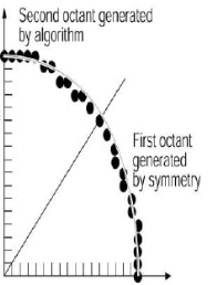
Q2) Write about clipping circles?

A6) Accept/Reject test

– Does the bounding box of the circle intersect with the clipping box?

●      If yes, condition pixel

Write on the clipping box inside/outside the test,

Also we can test Circle points by Point Clipping

- the point P=(x, y) is displayed in the clipping  Boundary if

Xmin< x <xmax and ymin<y<ymax

Q7) What is a polygon?

A7) A polygon is a surface representation. It is basic in nature and is closed. It is made up of a series of lines. It's also known as a multi-sided figure. Sides or edges are the lines that make up a polygon. Two vertices are combined to form the lines.

Example

●      Triangle

●      Rectangle

●      Hexagon

●      Pentagon

Some polygons are shown in the figures below.

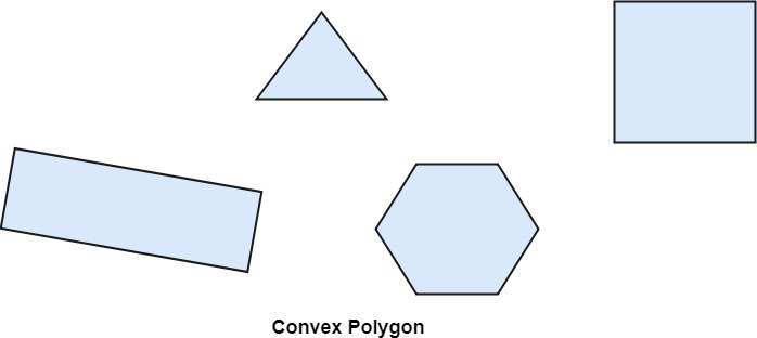
Fig 5: Example of polygon

Types of Polygons

●      Concave

●      Convex

When a line connecting any two inside points of a polygon lies inside the polygon, it is considered convex. Concave describes a non-convex polygon. One interior angle of a concave polygon is more than 180°. So that it can be cut into polygons that are comparable.

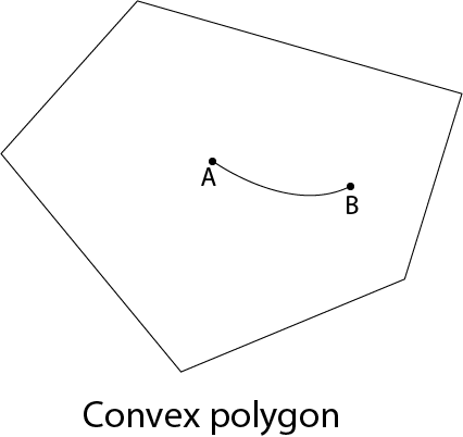
Fig 6: Convex polygon

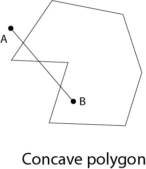
Fig 7: Concave polygon

A polygon can be orientated in either a positive or negative direction. The orientation is considered to be positive if we visit vertices and the vertices visit generates a counterclockwise circuit.

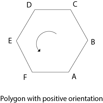
Fig 8: Polygon with positive orientation

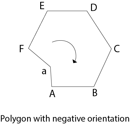
Fig 9: Polygon with negative orientation

Q8) Write about an ellipse?

A8) Ellipse is defined as the locus of a point in a plane that moves in such a way that the ratio of its distance from a fixed point called focus in the same plane to its distance from a fixed straight line called directrix is always constant and less than unity.

The general equation of the ellipse can be expressed as d1+d2=constant if the distance between the two foci from any point P=(x,y) on the ellipse is labeled d1 and d2.

We have the following formula for expressing the distances d1 and d2 in terms of focal coordinates F1 and F2:

Ax2+By2+Cxy+Dx+Ey+F=0 where A, B, C, D,E, and F are evaluated in terms of focal coordinates and dimensions of the major and minor axes of the ellipse.

Midpoint ellipse algorithm

The midpoint ellipse approach is used in two sections during the first quarter. Let's start at (0,ry) and work our way around the ellipse path in clockwise order in the first quadrant.

The ellipse function is defined as follows:

fellipse(x,y)=ry2x2+rx2y2-rx2ry2

The following are some of the properties that have been generated as a result of this:

●      fellipse(x,y)<0 which means (x,y) is inside the ellipse boundary.

●      fellipse(x,y)>0 which means (x,y) is outside the ellipse boundary.

●      fellipse(x,y)=0 which means (x,y) is on the ellipse boundary.

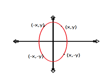
Initial decision parameter

Starting position = in area 1 yields the beginning value of a decision parameter (0,ry).

i.e. p10=ry2+1/4rx2-rx2ry

The initial position in region 2 is obtained from the last position selected in region 1, and the first decision parameter in region 2 is:

p20=ry2(x0+1/2)2+rx2(y0-1)2-rx2ry2

ALGORITHM

1. Take the input and ellipse centre and obtain the first point on an ellipse centered on the origin as a (x,y0)= (0,ry).
2. Now calculate the initial decision parameter in region 1 as:
   p10=ry2+1/4rx2-rx2ry
3. At each xk position in region 1 perform the following task. If p1k<0 then the next point along the ellipse centered on (0,0) is (xk+1,yk).
   i.e. p1k+1=p1k+2ry2xk+1+ry2

Otherwise the next point along the circle is (xk+1,yk -1)
i.e. p1k+1=p1k+2ry2xk+1 – 2rx2yk+1+ry2

4.     Now, again calculate the initial value in region 2 using the last point (x0,y0) calculated in a region 1 as) p20=ry2(x0+1/2)2+rx2(y0-1)2-rx2ry2

5.     At each yk position in region 2 starting at k =0 perform the following task. If p2k<0 the next point along the ellipse centered on (0,0) is (xk , yk-1)
i.e. p2k+1=p2k-2rx2yk+1+rx2

Otherwise the next point along the circle will be (xk+1,yk -1)
i.e. p2k+1 =p2k+2ry2xk+1 -2rx2yk+1+rx2

6.     Now determine the symmetric points in another three quadrants.

7.     Plot the coordinate value as: x=x+xc , y=y+yc

8.     Repeat the steps for region 1 until 2ry2x>=2rx2y.

Q9) Write the difference between cohen sutherland and liang barsky line algorithm?

A9) Difference between Cohen Sutherland and Liang Barsky Line algorithm

Q10) Let R be the rectangular window whose lower left-hand corner is at L (-3, 1) and upper right-hand corner is at R (2, 6). Find the region codes for the endpoints in fig:

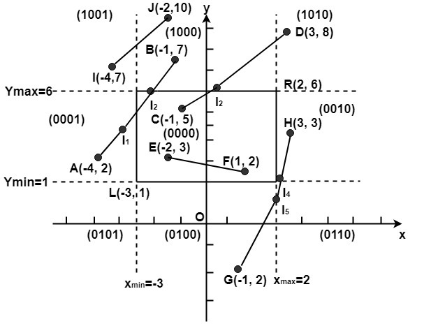
A10) The region code for point (x, y) is set according to the scheme

Bit 1 = sign (y-ymax)=sign (y-6)         Bit 3 = sign (x-xmax)= sign (x-2)

Bit 2 = sign (ymin-y)=sign(1-y)         Bit 4 = sign (xmin-x)=sign(-3-x)

Here

Line Clipping

So

A (-4, 2)→ 0001         F (1, 2)→ 0000

B (-1, 7) → 1000         G (1, -2) →0100

C (-1, 5)→ 0000         H (3, 3) → 0100

D (3, 8) → 1010         I (-4, 7) → 1001

E (-2, 3) → 0000         J (-2, 10) → 1000

We place the line segments in their appropriate categories by testing the region codes found in the problem.

Category1 (visible): EF since the region code for both endpoints is 0000.

Category2 (not visible): IJ since (1001) AND (1000) =1000 (which is not 0000).

Category 3 (candidate for clipping): AB since (0001) AND (1000) = 0000, CD since (0000) AND (1010) =0000, and GH. Since (0100) AND (0010) =0000.

The candidates for clipping are AB, CD, and GH.

In clipping AB, the code for A is 0001. To push the 1 to 0, we clip against the boundary line xmin=-3. The resulting intersection point is I1 (-3,3Line Clipping). We clip (do not display) AI1 and I1 B. The code for I1is 1001. The clipping category for I1 B is 3 since (0000) AND (1000) is (0000). Now B is outside the window (i.e., its code is 1000), so we push the 1 to a 0 by clipping against the line ymax=6. The resulting intersection is l2 (-1Line Clipping,6). Thus I2 B is clipped. The code for I2 is 0000. The remaining segment I1 I2 is displayed since both endpoints lie in the window (i.e., their codes are 0000).

For clipping CD, we start with D since it is outside the window. Its code is 1010. We push the first 1 to a 0 by clipping against the line ymax=6. The resulting intersection I3 is (Line Clipping,6),and its code is 0000. Thus I3 D is clipped and the remaining segment CI3 has both endpoints coded 0000 and so it is displayed.

For clipping GH, we can start with either G or H since both are outside the window. The code for G is 0100, and we push the 1 to a 0 by clipping against the line ymin=1.The resulting intersection point is I4 (2 Line Clipping,1) and its code is 0010. We clip GI4 and work on I4 H. Segment I4 H is not displaying since (0010) AND (0010) =0010.

For clipping CD, we start with D since it is outside the window. Its code is 1010. We push the first 1 to a 0 by clipping against the line ymax=6. The resulting intersection I3 is (Line Clipping,6), and its code is 0000. Thus I3 D is clipped and the remaining segment CI3 has both endpoints coded 0000 and so it is displayed.

For clipping GH, we can start with either G or H since both are outside the window. The code for G is 0100, and we push the 1 to a 0 by clipping against the line ymin=1.The resulting intersection point is I4 (2Line Clipping,1) and its code is 0010. We clip GI4 and work on I4 H. Segment I4 H is not displaying since (0010) AND (0010) =0010.