Unit 1 | unit 1 introduction and classification of signals

Unit - 1

Introduction and Classification of signals

Q1) What is a signal?

A1)

Definition: A signal is defined as a physical quantity that varies with time, space, or any other independent variable.

The signal may depend on one or more independent variables. If the signal depends on one variable, then it is known as a one-dimensional signal. If it depends on two independent variables, then the signal is known as a two-dimensional signal. Examples are pictures, X-ray images, and sonograms.

The multidimensional signal depends on many variables.

Q2) Explain the following signals?

Unit step function
Unit ramp function
Unit parabolic function
Unit impulse function

A2)

Unit step function

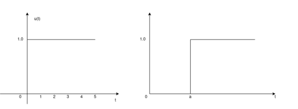
The unit step sequence is defined as:

u(t) = 1 for t

= 0 for t<0

From the above equation, we find the when the argument t in u(t) is less than zero then the unit step function is zero and when the argument t in u(t) is greater than or equal to zero then the unit step function is unity

Similarly, for a shifted unit step function u(t-a) is zero if the argument (t-a) <0 or t<a and is one of the argument (t-a) > 0 or t>a.

That is

u(t-a) = 1 for t>a

=0 for t<a

Unit ramp function

The unit ramp function is defined as:

r(t) = t for t

=0 for t<0

r(t) = t u(t)

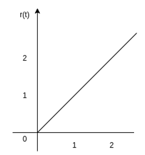
The ramp function can be obtained by applying the unit step function to an integrator.

r(t) = dt = ( in the time interval t>0)

The unit step function can be obtained by differentiating the unit ramp function

Thus

u(t) = d/dt r(t)

Unit parabolic function

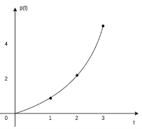
The unit parabolic function is given by

p(t) = t 2 / 2 for t 0

= 0 for t<0

p(t) = t2/2 u(t)

Impulse function

The impulse function occupies an important place in signal analysis. It is defined as

dt =1

And

δ(t) =0 for t

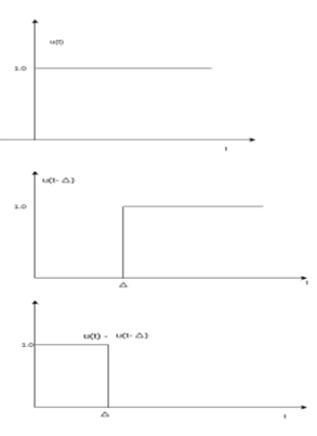
The impulse function has zero amplitude everywhere except at t=0. At t=0 the amplitude is infinity such that the area under the curve is equal to one. The unit impulse function can be obtained by using a limiting process on the rectangular pulse as shown in the figure.

Note that the area under the rectangular pulse is equal to unity.

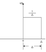
The rectangular pulse function of the figure can be expressed as

x(t) = 1/ ∆ [ u(t) – u(t-∆)] …………………………………..(1)

The impulse function can be obtained when the width ∆ ->0 that is

δ(t) = lim ∆-> 0 x(t)

= lim ∆-> 0 1/ ∆ [ u(t) – u(t-∆)]

The delayed unit impulse function is defined as

=1 for t=a

And =0 for t a

Q3) Explain sinusoidal signal and exponential signal, rectangular pulse?

A3)

Sinusoidal signal

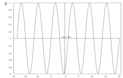
A continuous-time sinusoidal signal is given by

x(t) = A sin ( + ) ---------------------------------(1)

Where A is the amplitude, Ω is the frequency in radians per second, and is the phase angle in radians.

The figure shows the waveform of the sinusoidal signal with A=1, = -π/3 with period 2π/Ω.

Real exponential and complex exponential

Real exponential

A real exponential signal is defined as

x(t) = A e at --------------------------------(1)

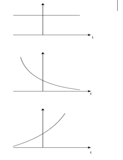
Where both A and a are real. Depending on the value of ‘a’ we get different signals. If ‘a’ is positive the signal x(t) is growing exponential as shown in fig(b) If ‘a’ is negative then x(t) is decaying exponential as shown in fig(c). For a=0 x(t) is constant.

Complex exponential signal

The most general for of complex exponential signal is given by

x(t) = e st ---------------------------------------(1)

Where s is a complex variable defined as

s = + j Ω

Therefore

x(t) = e st = e s( + j Ω) = e t . e j Ωt

Using Euler identity, we can expand

e j Ωt = cos Ω t + j sin Ωt

Substituting in eq(1) we get

x(t) = e t [ cos Ω t + j sin Ω t]

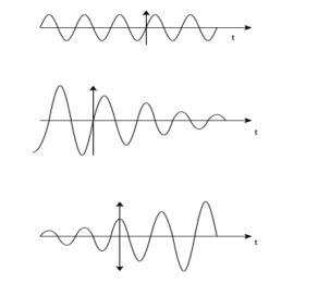
Depending on the values of and Ω we get different signals.

If =0 and Ω =0 x(t) = 1 that is the signal x(t) is a pure DC signal.
If Ω=0 then s = , x(t) = e t which decays exponentially for <0 and grows exponentially for > 0.
If =0 then s= jΩ gives x(t) = e j Ωt a sinusoidal signal with ɸ=0
If <0 with finite Ω we get an exponentially decaying sinusoidal signal.
If 0 with finite Ω we get an exponentially growing sinusoidal signal.

Rectangular Pulse:

The rectangular pulse function is defined as

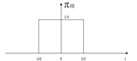
for |t| ½

=0 otherwise

Q4) Explain the Triangular pulse function, signum function, and gaussian function?

A4)

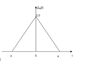
The unit triangular function is defined as

∆a(t) = 1 - |t|/a |t| a

0 |t| a

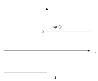
Signum function

The sinc function is defined by the expression

Sinc(t) = sin t/t -∞ < t < ∞

The sinc function oscillates with period 2π and decays with increasing t. Its value is zero at nπ , n = ±1, ±2,…………………….. It is an even function of t.

Gaussian function:

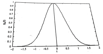
The Gaussian function is defined by the expression

Ga(t) = e – at ^2 - ∞ <t<∞

This function is extensively used in probability theory.

Q5) Explain time-shifting and time reversal?

A5)

Time Shifting

Let us consider a signal x(t) as shown in the figure. The time-shifting of x(t) may delay or advance the signal in time. Mathematically this can be represented by

y(t) = x(t-T) ------------------------------------------(1)

If T is positive the shifting delays the signal as shown in the figure.

If T is negative the shifting advances the signal as shown in the figure.

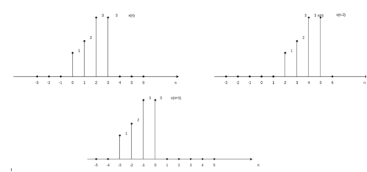
Similarly, the time-shifting operation of discrete-time signals is represented by

y(n) = x(n-k)

Which shows that the signal y(n) can be obtained by shifting x(n) by k units. If k is positive the shift is to the right (delay) and if k is negative the shift is to the left. Let us consider a signal x(n) as shown in the figure. The signal x(n-2) is obtained by shifting x(n-2) is obtained by shifting x(n) right by 2 units of time. The result is shown in fig (b). On the other hand x(n+3) is obtained by shifting x(n) left by three units of time.

Time Reversal

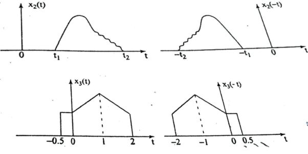
The time-reversal of signal x(t) can be obtained by folding the signal about t=0. It is denoted by x(-t). The signal x1(t) and its reflection x(-t) is illustrated in figs a and b respectively.

The signal x(-t+2) is obtained by delaying x1(-t) by two units of time and x1(-t-2) is obtained by advancing x1(-t) by two units of time. The signals x1(-t+2) and x1(-t-2) are shown in figure ( c) and (d).

The time-reversal of the discrete-time signal can be obtained by folding the sequence x(n) about n=0. For signal x1(n) in fig, the time-reversal signal x1(-n) is shown in fig (b).

The signal x1(-n+2) is obtained by delaying x1(-n) by two units of time and x1(-n-2) is obtained by advancing x1(-n) by two units of time. The other examples for time-reversal of a discrete-time signal are obtained by fig (a) and (b).

Q6) Explain amplitude scaling and time scaling?

A6)

Amplitude Scaling:

Consider a signal x(t) that is fed to an amplifier with a gain of 3 then the output of an amplifier can be represented by

y(t) = 3 x(t)

That is the output y(t) is identical in shape to the input signal x(t) but its amplitude is thrice everywhere. This concept is illustrated in the figure.

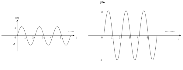
From fig we find that the amplitude is rescaled hence the name amplitude scaling.

Similarly, the amplitude scaling of a discrete-time signal can be represented by

y(n) = a x(n)

If x(n) is as shown in figure and a=2 then y(n) is as shown in figure(b).

Time scaling:

Let us consider a signal x(t) as shown in figure(a). The time scaling of a signal can be accomplished by replacing t by at in signal x(t).

If a=2 we get new signal

y(t) = x(2t)

Observe that x(t) is switching from 0 to 1 at t=-1 and switching from 1 to 0 at t=3. . When y(t) = 2t , y(t) = x(2t) , y(t) switches from 0 to 1 at t=0.5 and switches from 1 to 0 at t=1.5.

In the original signal x(t) magnitude is equal to 1 at t=0 and t=2. But in a time-scaled signal y(t) magnitude is equal to 1 at t=0 and t=2. But in a time-scaled signal y(t) magnitude is equal to 1 at t=0 and t=1. This behavior shows that x(t) is compressed in time by factor 2.

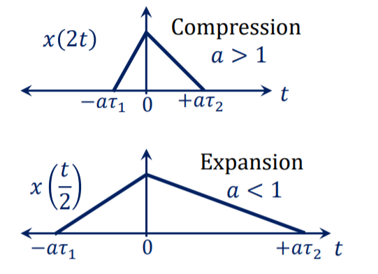
The resulting signal x(2t) is shown in fig(b). Let x(t) be an audio signal. If x(t) were recorded on a magnetic tape then x(2t) is the signal played back twice the recording speed.

Now consider another signal y(t) = x(at) with a=1/2. Figure ( c ) shows x(1/2) which is expanded in time by factor 2.

In discrete- time signal

y(n) = x(2n)

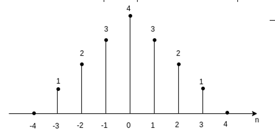
Let x(n) be a sequence as shown in figure. Then we plot time scaled signal y(n) by substituting different values of n.

For n =-1

y(-1) = x(-2) =2

…..

y(0) = x(0) =4

y(1) = x(2) =2

y(2) = x(4) = 0

Q7) Explain signal addition and multiplication?

A7)

Signal addition:

The sum of two continuous-time signals can be obtained by adding their values at every instant. Similarly, the subtractions of two continuous-time signals can be obtained by subtracting their values at every instant.

Let us consider the addition and subtraction of two signals x1(t) and x2(t) as shown in figure(a) and (b).

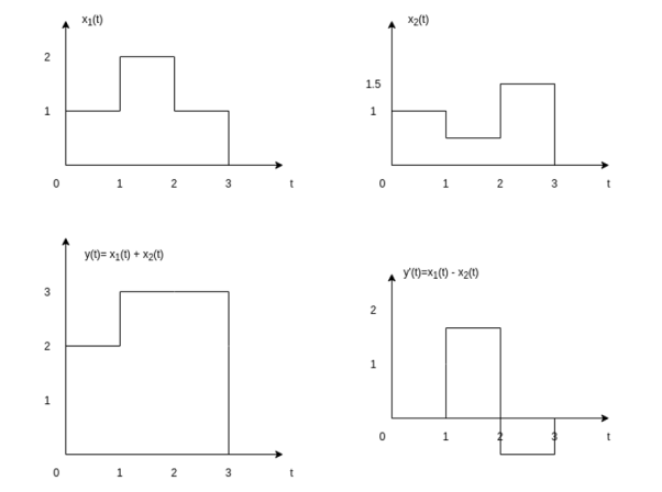
The addition of signals of two signals x1(t) and x2(t) can be obtained by considering each time interval separately as follows:

x1(t) = 1 for 0 t 1 and

x2(t) =1 for 0 t 1

Hence x1(t) + x2(t) = 2 for 0 t 1

x1(t) = 2 for 1 t 2 and

x2(t) =0.5 for 1 t 2

Hence x1(t) + x2(t) = 2.5 for 1 t 2

x1(t) = 1 for 2 t 3 and

x2(t) =1.5 for 2 t 3

Hence x1(t) + x2(t) = 2.5 for 2 t 3

The sketch for y(t) = x1(t) + x2(t) as shown in fig ( c )

In the same way the subtraction of x2(t) from x1(t) can be obtained. By inspection we can find

y’(t) = x1(t) – x2(t) = 0 for 0 t 1

= 1.5 for 1

= -0.5 for 2 t 3

For discrete-time signals, the sum of two sequences can be obtained by adding the sequence values at the same index n for which the sequences are defined.

If x1(n) = {1,3,2,1} and

x2(n) = {1,-2,3,2}

Then

x1(n) + x2(n) = { 1+1, 3-2,2+3,1+2}= {2,1,5,3}

x1(n) – x2(n) = { 1-1,3-(-2), 2-3, 1-2} = { 0,5,-1,-1}

Signal multiplication

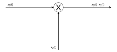
The multiplication of two signals can be obtained by multiplying their values at every instant.

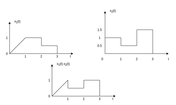
The multiplication process is illustrated in the figure.

In the interval 0 t 1

x1(t) = t; x2(t) = 1. Therefore y(t) = x1(t) x2(t)

Therefore y(t) = x1(t) x2(t)=t

In in the interval 1 t 2

x1(t) =1; x2(t) = 0.5. Therefore y(t) = 0.5

In in the interval 2 t 3

x1(t) =0.5; x2(t) = 1.5. Therefore y(t) = 0.75

Q8) Express the following:

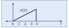
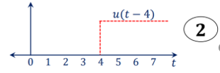
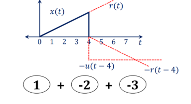
x(t) = r(t) – [ u(t-4) + r(t-4)]

A8)

Q9) Write a note on the classification of systems?

A9)

Static and Dynamic systems

A system is static or memoryless if its output at any instant of time depends on the input at that instant of time but not on the past or future values of input. Otherwise, the system is dynamic or with memory.

Casual and Non-casual systems

A causal system is one for which the output at any time depends on the present and past inputs but not future inputs These systems are known as non- anticipative systems.

A non-casual system is one whose output depends on future values.

Linear and Non-linear systems

The superposition principle states that the response to a weighted sum of input signals be equal to the weighted sum of the outputs corresponding to each of the individual input signals. A system that satisfies the superposition principle is said to be the linear system.

T [a1 x1(t) + a2 x2(t)] = a1 T[x1(t)] + a2 T[x2(t)]

∴, T [a1 x1(t) + a2 x2(t)] = a1 y1(t) + a2 y2(t)

Similarly, for discrete –time linear system

T [ax1(n) + bx2(n)] = a T[x1(n) + bTx2(n)]

Time Variant and Time invariant systems

A system is said to be time-variant if its input-output characteristics do not change with time.

Suppose we apply a signal(t) to a system to a system and obtain an output y(t) as shown in the figure.

If we delay by T seconds then for a time-invariant system the output will be delayed by T seconds.

Stable and unstable systems.

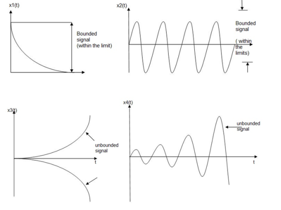
An input signal x(t) is said to be bounded if it satisfies the condition |x(t) |≤Mx < ∞ for all t.

Similarly, the output signal is bounded if it satisfies the condition |y(t)| ≤My < ∞

The example for bounded and unbounded signals is as shown in the figure.

Note: For a bounded signal, the amplitude is finite.

Q10) Check whether the following systems are

 Static or dynamic

 Linear or Non-linear

 Causal or non-casual

 Time-Invariant or time-variant

A10)

a) y(t) d2y(t) /dt2 + 3t dy(t)/dt + y(t) = x(t)

Since it is a differential equation the system is dynamic.
The input x1(t) and output y1(t) can be described by

y1(t) d2 y1(t)/dt2 + 3t dy1(t)/dt + y1(t) = x1(t)

Similarly, y2(t) d2y2(t)/dt2 + 3t dy2(t)/dt + y2(t) =x2(t)

a y1(t) d2y1(t)/dt2 + 3at dy1(t)/dt + a y1(t) + b y2(t) d2y1(t)/dt2 + 3bt dy1(t)/dt +by2(t) = ax1(t) + b x2(t)

Ay1 d2 y1(t)/dt2 + by2(t) d2 y(t)/dt2 + 3t d/dt[ay1(t) + b2 y2(t)] + ay1(t) + b y2(t) = ax1(t) + bx2(t)

Since the differentiation ay1(t) d2 y1(t)/dt2 + by2(t) d2 y2(t)/dt2 is not a function of the weighted sum of outputs, superposition principle is not satisfied hence the system is non-linear.

The output depends on the present input only hence the system is causal.
The co-efficient of the differential equations is a function of time. Hence the system is time-variant.

y(n) = x(n) x(n-1)

The output depends on the past values of input. Hence it requires memory therefore the system is dynamic.

The output y1(n) for input x1(n) is

y1(n) = x1(n) x1(n-1)

y2(n) = x2(n) x2(n-1)

y3(n) = ax1(n) + b x2(n) [ax1(n-1) + b x2(n-1)]

a y1(n) + by2(n) = a x1(n) x1(n-1) + bx2(n) x2(n-1)

Since y3(n) ≠ ay1(n) + b y2(n)

Hence the system is non-linear.

The output depends on the present and past values of input. Hence the system is casual.

y(n) = x(n) x(n-1)

y (n, k) = x(n-k) x(n-1-k)

y(n-k) = x(n-k) x(n-1-k)

Since y(n, k) = y(n-k) the system is time-invariant.

b) y (n) = cos[x(n)]

The output depends on the input at that instant. Therefore, system is static.

For input x1(n)

y1(n) = cos[x1(n)]

For input x2(n)

y2(n) = cos[x2(n)]

y3(n) = cos[ax1(n)+ b x2(n)]

a y1(n) + b y2(n) = a cos [x1(n)] + b cos[x2(n)]

Hence the system is non-linear.

The output depends on the present input hence the system is casual.

y(n) = cos[x(n)]

y(n, k) = cos[x(n-k)]

y(n-k) = cos[x(n-k)]

y(n, k) = y(n-k)

Hence system is time –invariant.

For the given system check whether the system is linear, time-invariant, casual memoryless, or stable.

y(t) = x(t-2) + x(2-t)

The system is not memoryless since the output depends on the past and future values of input.
The system is non-casual since output depends on the future values of input.

y (t, = x1(t-2-)+x1(2-t-)

y(t-) = x(t-2-) + x2(2-t+)

y (t, ≠ y (t-

System is time variant.

y1(t) = x1(t-2) + x1(2-t)

y2(t) = x2(t-2) + x2(2-t)

a1y1(t) + a2 y2(t) = a1 x1(t-2)+ a1x1(2-t) + a2x2(t-2)+a2x2(2-t)

= a1x1(t-2) + ax2(t-2) +a1x1(2-t)+a2 x2(2-t)

= System is linear.

For bounded input, the output is also bounded. Hence the system is stable.

Q11) Sketch the continuous-time signal x(t) = 2 sin πt for interval 0 2. Sample the continuous-time signal with a sampling period T =0.2 sec and sketch the discrete-time signal.

A11)

Given:

x(t) = 2 sin πt

To sketch the signal we have values x(t) for different values of t, that is

x(0) = 2 sin π (0) = 0.

x(0.25) = 2 sin π (0.25) = √2

x(0.5) = 2 sin π (0.5) = 2

x(0.75) = 2 sin π (0.75) = √2.

x(1) = 2 sin π (1) = 0

x(1.25) = 2 sin π (1.25 = -√2

x(1.5) = 2 sin π (1.5) = -2.

x(0.25) = 2 sin π (1.75) = - √2

x(2) = 2 sin 2π =0

Take t on x-axis and x(t) on y-axis. Mark the above points and join all the points by a smooth curve to get continuous signal as shown in fig (a) . Given sampling period T =0.2

Q12) Sketch the signal x(t) = e -t for an interval 0 t 2