Unit - 1
Introduction to Signals and Systems
Q1) Explain Periodicity?
A1) The signal’s behaviour/graph repeats after every T. Therefore,
x(t) = x(t + nT) or
x(t) = x(t – nT)
Where, T is the fundamental period. So we can say that the signal remains unchanged when shifted by multiples of T.
Q2) Differentiate between deterministic and non determinstic signal?
A2)
Deterministic
A signal is said to be deterministic if there is no uncertainty with respect to its value at any instant of time or the signals which can be defined exactly by a mathematical formula are known as deterministic signals.

Fig. Deterministic signal
Random
A signal is said to be non-deterministic(stochastic) if there is uncertainty with respect to its value at some instant of time. Non-deterministic signals are random in nature hence they are called random signals. Random signals cannot be described by a mathematical equation. They are modelled in probabilistic terms.

Fig. Random signal
Q3) Explain unit step sequence and unit impulse sequence?
A3) Unit step sequence:
The unit step sequence is defined as:
u(n) = 1 for n 
=0 for n<0

Figure. Unit Step Signal
Unit Impulse
The impulse function occupies an important place in signal analysis. It is defined as
 dt =1
dt =1
And
δ(t) =0 for t
The impulse function has zero amplitude everywhere except at t=0. At t=0 the amplitude is infinity such that the area under the curve is equal to one. The unit impulse function can be obtained by using limiting process on the rectangular pulse as shown in figure.
Note that the area under the rectangular pulse is equal to unity.
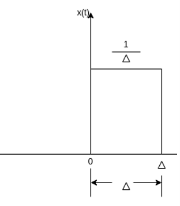
Fig. Impulse function
The rectangular pulse function of the figure can be expressed as
x(t) = 1/ ∆ [ u(t) – u(t-∆)] …………………………………..(1)
The impulse function can be obtained when the width ∆ ->0 that is
δ(t) = lim ∆-> 0 x(t)
= lim ∆-> 0 1/ ∆ [ u(t) – u(t-∆)]

Fig. Unit impulse with delay function
The delayed unit impulse function is defined as
 =1 for t=a
And  =0 for t
 a
a
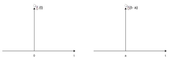
Fig. Impulse function
Q4) Explain Continuous and Discrete time signal?
A4) A continuous time system is one which operates on the continuous time input signal and produces a continuous-time output signal.

Figure. I/O of continuous time signal
If the input is x(t) and output is y(t) then
y(t) = T{x(t)}
That is x(t ) is transformed to y(t).
Example : Amplifiers, filters, motors etc
Discrete time system is one which operates on discrete time input signal and produces a discrete-time output signal.

Figure. I/O of Discrete time signal
If the input is x(n) and output y(n) then
y(n) = T[x(n)]
Q5) Explain Linearity property?
A5) Constitutes two properties:
Additivity/ Super position
If x1(t) -> y1(t)
And x2(t) -> y2(t)
Then
x1(t) + x2(t) -> y1(t) + y2(t)
Property of scaling
If x1(t) -> y1(t)
a * x1(t) -> a * y1(t)
If both are satisfied, then system is linear
y(t) = x2(t)
The responses due to inputs x1(t) and x2(t) are given by
y1(t) = x1 2(t)
y2(t) = x2 2(t)
The output due to weighted sum of inputs is
y3(t) = T[ax1(t) + bx2(t)] = [ax1(t) + bx2(t)]2
The weighted sum of inputs
a y1(t) + by2(t) = ax12(t) + b x2 2(t)
y3(t) ≠ ay1(t) + by2(t)
System is non-linear.
Q6) Explain additive and homogeneity property?
A6) Homogeneity
Homogeneity means change in input signals amplitude results in a corresponding change in the output signal’s amplitude.
That is a change in x[n] will result in a change in y [n]
Also, a change in k x[n] will result in a change in k y[n]
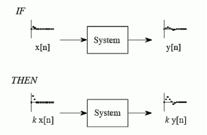
Figure. Homogenity
Additivity
Consider a system where input x1[n] produces an output y1[n]. Similarly x2[n] produces y2[n].
The system is additive when
x1[n] + x2[n] = y1[n] + y2[n]
In other words signals added at the input will produce signals added at the output.
Q7) Explain Shift invariance property?
A7) Shift invariance means that a shift in the input signal will result in an identical shift in the output signal
If x[n] -> y[n]
Then x[n+s] -> y[n +s] for any constant s
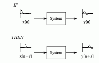
Figure. Shift Invariance
Q8) Explain causality property?
A8) The property of causality is a requirement for a system to be realizable in reality. Causality means that the output of the system does not depend on future inputs, but only on past input.
Examples of casual system:
y(t) = x(t) + x(t-1)
y(n) = n x(n) + x(n-3)
Examples of non-casual system
y(t) = x(t+3) + x 2 (t)
y(n) = x(2n)
For example
y(t) = 2 x(t) + 3 x(t-3)
Let t=1 therefore y (1) = 2 x(1) + 3 x(-2)
The system output only depends upon present and past inputs. Hence, the system is causal.
y(t) = 2 x(t) + 3 x(t – 3) + 6 x( t+3)
Let t=1 the system output is
y(1) = 2x(1) + 3 x(-2) + 6 x( 4)
Here the output depends future input. Hence non –casual.
Q9) Explain the property of stability?
A9) Figure Stability of the system
An input signal x(t) is said to be bounded if it satisfies the condition |x(t) |≤Mx < ∞ for all t.
Similarly, the output signal is bounded if it satisfies the condition |y(t)| ≤My < ∞
The example for bounded and unbounded signals is as shown in the figure.
Note: For a bounded signal, the amplitude is finite.
Example 1: y (t) = x2(t)
Let the input is u(t) that is unit step then output y(t) = u2(t) = u(t) = bounded output.
Hence, the system is stable.
Example 2: y (t) = ∫x(t)dt∫x(t)dt
Let the input be u (t) then
Output y(t) = ∫u(t)dt but ∫ u(t)dt = ramp signal
It is unbounded because the amplitude of ramp is not finite and tends to become infinite when t →infinite
Hence, the system is unstable.
Q10) Explain Realizability?
A10) Consider the first system,
y(t)=x(t−1)y(t)=x(t−1) is a causal system, because its output is a time-delayed version of the original signal.
On the other hand, the second system y(t)=x(t+1)y(t)=x(t+1), is non-causal.
This system returns a time-advanced version of the input signal. This means, that for example at the output time t=0, the system requires access to the value of the input signal at time t=1. Clearly, this is impossible in a realizable system, as nobody can predict the future.
Unit - 1
Introduction to Signals and Systems
Q1) Explain Periodicity?
A1) The signal’s behaviour/graph repeats after every T. Therefore,
x(t) = x(t + nT) or
x(t) = x(t – nT)
Where, T is the fundamental period. So we can say that the signal remains unchanged when shifted by multiples of T.
Q2) Differentiate between deterministic and non determinstic signal?
A2)
Deterministic
A signal is said to be deterministic if there is no uncertainty with respect to its value at any instant of time or the signals which can be defined exactly by a mathematical formula are known as deterministic signals.
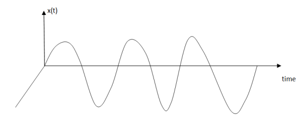
Fig. Deterministic signal
Random
A signal is said to be non-deterministic(stochastic) if there is uncertainty with respect to its value at some instant of time. Non-deterministic signals are random in nature hence they are called random signals. Random signals cannot be described by a mathematical equation. They are modelled in probabilistic terms.

Fig. Random signal
Q3) Explain unit step sequence and unit impulse sequence?
A3) Unit step sequence:
The unit step sequence is defined as:
u(n) = 1 for n 
=0 for n<0

Figure. Unit Step Signal
Unit Impulse
The impulse function occupies an important place in signal analysis. It is defined as
 dt =1
dt =1
And
δ(t) =0 for t
The impulse function has zero amplitude everywhere except at t=0. At t=0 the amplitude is infinity such that the area under the curve is equal to one. The unit impulse function can be obtained by using limiting process on the rectangular pulse as shown in figure.
Note that the area under the rectangular pulse is equal to unity.

Fig. Impulse function
The rectangular pulse function of the figure can be expressed as
x(t) = 1/ ∆ [ u(t) – u(t-∆)] …………………………………..(1)
The impulse function can be obtained when the width ∆ ->0 that is
δ(t) = lim ∆-> 0 x(t)
= lim ∆-> 0 1/ ∆ [ u(t) – u(t-∆)]
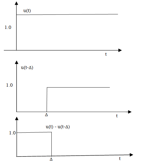
Fig. Unit impulse with delay function
The delayed unit impulse function is defined as
 =1 for t=a
And  =0 for t
 a
a

Fig. Impulse function
Q4) Explain Continuous and Discrete time signal?
A4) A continuous time system is one which operates on the continuous time input signal and produces a continuous-time output signal.

Figure. I/O of continuous time signal
If the input is x(t) and output is y(t) then
y(t) = T{x(t)}
That is x(t ) is transformed to y(t).
Example : Amplifiers, filters, motors etc
Discrete time system is one which operates on discrete time input signal and produces a discrete-time output signal.

Figure. I/O of Discrete time signal
If the input is x(n) and output y(n) then
y(n) = T[x(n)]
Q5) Explain Linearity property?
A5) Constitutes two properties:
Additivity/ Super position
If x1(t) -> y1(t)
And x2(t) -> y2(t)
Then
x1(t) + x2(t) -> y1(t) + y2(t)
Property of scaling
If x1(t) -> y1(t)
a * x1(t) -> a * y1(t)
If both are satisfied, then system is linear
y(t) = x2(t)
The responses due to inputs x1(t) and x2(t) are given by
y1(t) = x1 2(t)
y2(t) = x2 2(t)
The output due to weighted sum of inputs is
y3(t) = T[ax1(t) + bx2(t)] = [ax1(t) + bx2(t)]2
The weighted sum of inputs
a y1(t) + by2(t) = ax12(t) + b x2 2(t)
y3(t) ≠ ay1(t) + by2(t)
System is non-linear.
Q6) Explain additive and homogeneity property?
A6) Homogeneity
Homogeneity means change in input signals amplitude results in a corresponding change in the output signal’s amplitude.
That is a change in x[n] will result in a change in y [n]
Also, a change in k x[n] will result in a change in k y[n]

Figure. Homogenity
Additivity
Consider a system where input x1[n] produces an output y1[n]. Similarly x2[n] produces y2[n].
The system is additive when
x1[n] + x2[n] = y1[n] + y2[n]
In other words signals added at the input will produce signals added at the output.
Q7) Explain Shift invariance property?
A7) Shift invariance means that a shift in the input signal will result in an identical shift in the output signal
If x[n] -> y[n]
Then x[n+s] -> y[n +s] for any constant s

Figure. Shift Invariance
Q8) Explain causality property?
A8) The property of causality is a requirement for a system to be realizable in reality. Causality means that the output of the system does not depend on future inputs, but only on past input.
Examples of casual system:
y(t) = x(t) + x(t-1)
y(n) = n x(n) + x(n-3)
Examples of non-casual system
y(t) = x(t+3) + x 2 (t)
y(n) = x(2n)
For example
y(t) = 2 x(t) + 3 x(t-3)
Let t=1 therefore y (1) = 2 x(1) + 3 x(-2)
The system output only depends upon present and past inputs. Hence, the system is causal.
y(t) = 2 x(t) + 3 x(t – 3) + 6 x( t+3)
Let t=1 the system output is
y(1) = 2x(1) + 3 x(-2) + 6 x( 4)
Here the output depends future input. Hence non –casual.
Q9) Explain the property of stability?
A9) Figure Stability of the system
An input signal x(t) is said to be bounded if it satisfies the condition |x(t) |≤Mx < ∞ for all t.
Similarly, the output signal is bounded if it satisfies the condition |y(t)| ≤My < ∞
The example for bounded and unbounded signals is as shown in the figure.
Note: For a bounded signal, the amplitude is finite.
Example 1: y (t) = x2(t)
Let the input is u(t) that is unit step then output y(t) = u2(t) = u(t) = bounded output.
Hence, the system is stable.
Example 2: y (t) = ∫x(t)dt∫x(t)dt
Let the input be u (t) then
Output y(t) = ∫u(t)dt but ∫ u(t)dt = ramp signal
It is unbounded because the amplitude of ramp is not finite and tends to become infinite when t →infinite
Hence, the system is unstable.
Q10) Explain Realizability?
A10) Consider the first system,
y(t)=x(t−1)y(t)=x(t−1) is a causal system, because its output is a time-delayed version of the original signal.
On the other hand, the second system y(t)=x(t+1)y(t)=x(t+1), is non-causal.
This system returns a time-advanced version of the input signal. This means, that for example at the output time t=0, the system requires access to the value of the input signal at time t=1. Clearly, this is impossible in a realizable system, as nobody can predict the future.