undefined | unit 3 correlation

Unit – 3

Correlation

Q1) Compute Pearsons coefficient of correlation between advertisement cost and sales as per the data given below:

Advertisement cost	39	65	62	90	82	75	25	98	36	78
sales	47	53	58	86	62	68	60	91	51	84

A1)

X	Y	X - X	(X - X)2	Y - Y	(Y - Y)2
39	47	-26	676	-19	361	494
65	53	0	0	-13	169	0
62	58	-3	9	-8	64	24
90	86	25	625	20	400	500
82	62	17	289	-4	16	-68
75	68	10	100	2	4	20
25	60	-40	1600	-6	36	240
98	91	33	1089	25	625	825
36	51	-29	841	-15	225	435
78	84	13	169	18	324	234
650	660		5398		2224	2704

r = (2704)/√5398 √2224 = (2704)/(73.2*47.15) = 0.78

Thus Correlation coefficient is positively correlated

Q2) Compute correlation coefficient from the following data.

Hours of sleep (X)	Test scores (Y)
8	81
8	80
6	75
5	65
7	91
6	80

A2)

X	Y	X - X	(X - X)2	Y - Y	(Y - Y)2
8	81	1.3	1.8	2.3	5.4	3.1
8	80	1.3	1.8	1.3	1.8	1.8
6	75	-0.7	0.4	-3.7	13.4	2.4
5	65	-1.7	2.8	-13.7	186.8	22.8
7	91	0.3	0.1	12.3	152.1	4.1
6	80	-0.7	0.4	1.3	1.8	-0.9
40	472		7		361	33

X = 40/6 =6.7

Y = 472/6 = 78.7

r = (33)/√7 √361 = (33)/(2.64*19) = 0.66

Thus Correlation coefficient is positively correlated

Q3) Calculate coefficient of correlation between X and Y series using Karl pearson shortcut method.

X	14	12	14	16	16	17	16	15
Y	13	11	10	15	15	9	14	17

A3)

Let assumed mean for X = 15, assumed mean for Y = 14

X	Y	dx	dx2	dy	dy2	dxdy
14	13	-1.0	1.0	-1.0	1.0	1.0
12	11	-3.0	9.0	-3.0	9.0	9.0
14	10	-1.0	1.0	-4.0	16.0	4.0
16	15	1.0	1.0	1.0	1.0	1.0
16	15	1.0	1.0	1.0	1.0	1.0
17	9	2.0	4.0	-5.0	25.0	-10.0
16	14	1	1	0	0	0
15	17	0	0	3	9	0
120	104	0	18	-8	62	6

r = 8 *6 – (0)*(-8)

√8*18-(0)2 √8*62 – (-8)2

r = 48/√144*√432 = 0.19

Q4) Calculate coefficient of correlation between X and Y series using Karl pearson shortcut method.

X	1800	1900	2000	2100	2200	2300	2400	2500	2600
F	5	5	6	9	7	8	6	8	9

A4)

Assumed mean of X and Y is 2200, 6

X	Y	dx	dx (i=100)	dx2	dy	dy2	dxdy
1800	5	-400	-4	16	-1.0	1.0	4.0
1900	5	-300	-3	9	-1.0	1.0	3.0
2000	6	-200	-2	4	0.0	0.0	0.0
2100	9	-100	-1	1	3.0	9.0	-3.0
2200	7	0	0	0	1.0	1.0	0.0
2300	8	100	1	1	2.0	4.0	2.0
2400	6	200	2	4	0	0	0.0
2500	8	300	3	9	2	4	6.0
2600	9	400	4	16	3	9	12.0

			0	60	9	29	24

Note – we can also proceed dividing x/100

r = (9)(24) – (0)(9)

√9*60-(0)2 √9*29– (9)2

r = 0.69

Q5) Calculate Spearman rank-order correlation.

Test 1	8	7	9	5	1
Test 2	10	8	7	4	5

A5)

Here, highest value is taken as 1

Test 1	Test 2	Rank T1	Rank T2	d	d2
8	10	2	1	1	1
7	8	3	2	1	1
9	7	1	3	-2	4
5	4	4	5	-1	1
1	5	5	4	1	1
					8

R = 1 – (6*8)/5(52 – 1) = 0.60

Q6) Calculate Spearman rank-order correlation.

English	56	75	45	71	62	64	58	80	76	61
Maths	66	70	40	60	65	56	59	77	67	63

A6)

Rank by taking the highest value or the lowest value as 1.

Here, highest value is taken as 1

English	Maths	Rank (English)	Rank (Math)	d	d2
56	66	9	4	5	25
75	70	3	2	1	1
45	40	10	10	0	0
71	60	4	7	-3	9
62	65	6	5	1	1
64	56	5	9	-4	16
58	59	8	8	0	0
80	77	1	1	0	0
76	67	2	3	-1	1
61	63	7	6	1	1
					54

R = 1-(6*54)

10(102-1)

R = 0.67

Therefore this indicates a strong positive relationship between the ranks individuals obtained in the math and English exam.

Q7) Find Spearman's rank correlation coefficient between X and Y for this set of data:

X	13	20	22	18	19	11	10	15
Y	17	19	23	16	20	10	11	18

A7)

X	Y	Rank X	Rank Y	d	d2
13	17	3	4	-1	1
20	19	7	6	1	1
22	23	8	8	0	0
18	16	5	3	2	2
19	20	6	7	-1	1
11	10	2	1	1	1
10	11	1	2	-1	1
15	18	4	5	-1	1
					8

R =

R = 1 – 6*8/8(82 – 1) = 1 – 48 = 0.90

504

Q8) Find Spearman's rank correlation coefficient:

Commerce	15	20	28	12	40	60	20	80
Science	40	30	50	30	20	10	30	60

A8)

C	S	Rank C	Rank S	d	d2
15	40	2	6	-4	16
20	30	3.5	4	-0.5	0.25
28	50	5	7	-2	4
12	30	1	4	-3	9
40	20	6	2	4	16
60	10	7	1	6	36
20	30	3.5	4	-0.5	0.25
80	60	8	8	0	0
					81.5

R = 1 – (6*81.5)/8(82 – 1) = 0.02

Q9) Explain regression analysis.

A9)

Regression analysis is a technique of studying the dependence of one variable called dependent variable, on one or more variable called explanatory variable, with a view to estimate or predict the average value of the dependent variables in terms of the known or fixed values of the independent variables.

Regression analysis includes several variations, such as linear, multiple linear, and nonlinear. The most common models are simple linear and multiple linear.

Nonlinear regression analysis is commonly used for more complicated data sets in which the dependent and independent variables show a nonlinear relationship.

Linear model assumption -

The dependent and independent variables show a linear relationship between the slope and intercept.

The independent variable is not random.

The value of the residual (error) is zero.

The value of the residual (error) is constant across all observations.

The value of the residual (error) is not correlated across all observations.

The residual (error) values follow the normal distribution.

Importance

Regression Analysis, a statistical technique, is used to evaluate the relationship between two or more variables. Regression analysis helps an organisation to understand what their data points represent and use them accordingly with the help of business analytical techniques in order to do better decision-making. In this analysis, you will understand how the typical value of the dependent variable changes when one of the independent variables is varied, while the other independent variables are held fixed. Business analysts and data professionals use this powerful statistical tool for removing the unwanted variables and select the important ones.

Q10) How to find a linear regression equation.

Subject	X	Y
1	43	99
2	21	65
3	25	79
4	42	75
5	57	87
6	59	81

A10)

Subject	X	Y	Xy	X2	Y2
1	43	99	4257	1849	9801
2	21	65	1365	441	4225
3	25	79	1975	625	6241
4	42	75	3150	1764	5625
5	57	87	4959	3249	7569
6	59	81	4779	3481	6521
Total	247	486	20485	11409	40022

To find a and b, use the following equation

Find a:

((486 × 11,409) – ((247 × 20,485)) / 6 (11,409) – 247*247)

484979 / 7445

=65.14

Find b:

(6(20,485) – (247 × 486)) / (6 (11409) – 247*247)

(122,910 – 120,042) / 68,454 – 2472

2,868 / 7,445

= .385225

y’ = a + bx

y’ = 65.14 + .385225x

Q11) Calculate linear regression analysis.

Students	X	Y
1	95	85
2	85	95
3	80	70
4	70	65
5	60	70

A11)

students	X	Y	X2	y2	xy
1	95	85	9025	7225	8075
2	85	95	7225	9025	8075
3	80	70	6400	4900	5600
4	70	65	4900	4225	4550
5	60	70	3600	4900	4200
total	390	385	31150	30275	30500

To find a and b, use the following equation

Find a:

((385 × 31150) – ((390 × 30500)) / 5 (31150) – 152100)

97750 / 3650

=26.78

Find b:

(5(30500) – (390 × 385)) / (5 (31150) – 152100)

2,350 / 3650

= .0.64

y’ = a + bx

y’ = 26.78 + .0.64x

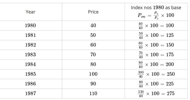
Q12) From the following data of wholesale prices of wheat for ten years construct index number taking a) 1998 as base and b) by chain base method.

Q13) From the following data calculate the index numbers using the Chain Index Numbers method.

Year 2011 2012 2013 2014 2015 2016 2017 2018

Prices 120 124 130 144 150 160 164 170

A13)

Construction of Chain Index Numbers

Year	Price	Link Relatives	Chain indices
2011	120	100	100
2012	124	120/124 x 100 = 103.33	103.33 ×100/100 = 103.33
2013	130	124/130 x 100 = 104.83	104.83 ×103.33/100 = 108.32
2014	144	130/144 x 100 = 110.76	110.76×108.32 /100= 119.98
2015	150	144/150 x 100 = 104.16	104.16 ×119.98/100 = 124.97
2016	160	150/160 x 100 = 106.66	106.66×124.97/100 = 133.29
2017	164	160/164 x 100 = 102.5	102.5 ×133.29/100 = 136.62
2018	170	164/170 x 100 = 103.65	103.65 ×136.62/100 = 141.61

Q14) Compute the chain base index numbers-

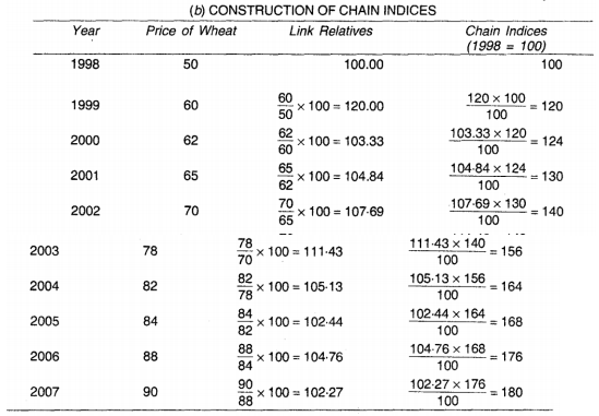
A14)

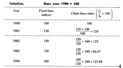
Q15) Find index numbers for the following data taking 1980 as the base year.

Year	1980	1981	1982	1983	1984	1985	1986	1987
Price	40	50	60	70	80	100	90	110

A15)

Q16) Find the index number from the data given below.

Commodities	Units	Price in 2007	Price in 2008
Sugar	Quintal	2200	3200
Milk	Quintal	18	20
Oil	Liter	68	71
Wheat	Quintal	900	1000
Clothing	Meter	50	60

A16)

Commodities	Units	Price in 2007	Price in 2008
Sugar	Quintal	2200	3200
Milk	Quintal	18	20
Oil	Liter	68	71
Wheat	Quintal	900	1000
Clothing	Meter	50	60
		= 3236	= 4351

Index number ( P01 ) =

P01 = (4351/3236)*100 = 134.45

It means the price in 2008 were 34% more than the price in 2007

Q17) Construct the price index for 2003, taking the year 2000 as base year.

Commodities	Price in 2000	Price in 2003
A	60	80
B	50	60
C	70	100
D	120	160
E	100	150

A17)

Commodities	Price in 2000 - P 0	Price in 2003 - P 1
A	60	80
B	50	60
C	70	100
D	120	160
E	100	150
	= 400	= 550

Index number ( P01 ) =

P01 = (550/400)*100 = 137.5

Therefore there is an increase of 37.5% in the prices in 2003 as against 2000.

Q18) Prepare simple aggregative price index.

Commodities	Price in 1995 - P 0	Price in 2003 - P 1
Wheat	100	140
Rice	200	250
Pulses	250	350
Sugar	14	20
Oil	40	50

A18)

Commodities	Price in 1995 - P 0	Price in 2003 - P 1
Wheat	100	140
Rice	200	250
Pulses	250	350
Sugar	14	20
Oil	40	50
	= 604	= 810

Simple aggregative index number = (810/604)*100 = 134.1

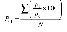
Q19) Using simple average of price relative method find price index for 2010, taking 2009 as base year for the following data.

Commodities	Price (2009)	Price(2010)
A	60	80
B	50	60
C	60	72
D	50	75
E	25	37 .5
F	20	30

A19)

Commodities	Price (2009)	Price(2010)	Price relatives
A	60	80	133.33
B	50	60	120
C	60	72	120
D	50	75	150
E	25	37 .5	150
F	20	30	150
N = 6			823.33

= 823.33/6 = 137.22

Q20) Calculate the price indices from the following data by applying (1) Laspeyre’s method (2) Paasche’s method and (3) Fisher ideal number by taking 2010 as the base year.

Commodity	2010		2011
Commodity	PO	QO	P1	Q1
A	20	10	25	13
B	50	8	60	7
C	35	7	40	6
D	25	5	35	4

A20)

Commodity	2010		2011
Commodity	PO	QO	P1	Q1	Poqo	P1qo	Poq1	P1q1
A	20	10	25	13	200	250	260	325
B	50	8	60	7	400	480	350	420
C	35	7	40	6	245	280	210	240
D	25	5	35	4	125	175	100	140
					970	1185	920	1125

Laspeyre’s formula-

P 01 = (1185/970)*100 = 122.16

Paasche’s formula-

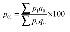
P 01 = (1125/920)*100 = 122.28

Fisher’s ideal formula-

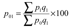
P 01 = √ = ((1185/970) + (1125/920)) *100 = 120.55

Sign Up