UNIT 3

IMAGE RESTORATION

Q1) Explain thresholding in Inverse filtering

A1)

Thresholding

We can model a blurred image by

Where f is the original image, b is some kind of a low pass filter and g is our blurred image. So to get back the original image, we would just have to convolve our blurred function with some kind of a high pass filter

But how do we find h? If we take the DFT of b so that B=DFT2(b), we would get something that looks like this

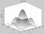
In the ideal case, we would just invert all the elements of B to get a high pass filter. However, notice that a lot of the elements in B have values either at zero or very close to it. Inverting these elements would give us either infinities or some extremely high values. To avoid these values, we will need to set some sort of a threshold on the inverted element. So instead of making a full inverse out of B, we can an "almost" full inverse by

So the higher we set , the closer H is to the full inverse filter.

Implementation and Results

Since Matlab does not deal well with infinity, we had to threshold B before we took the inverse. So we did the following:

Where n is essentially and is set arbitrarily close to zero for noiseless cases. The following images show our results for n=0.0001.

We see that the image is almost exactly like the original. The MSE is 2.5847.

Because an inverse filter is a high pass filter, it does not perform well in the presence of noise. There is a definite tradeoff between de-blurring and de-noising. In the following image, the blurred image is corrupted by AWGN with a variance of 10. n=0.2.

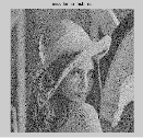
The MSE for the restored image is 1964.5. We can see that the sharpness of the edges improved but we also have a lot of noise specs in the image. We can get rid of more specs (thereby getting a smoother image) by increasing n. In general, the more noise we have in the image, the higher we set n. The higher the n, the less high pass the filter is, which means that it amplifies noiseless. It also means, however, that the edges will not be as sharp as they could be.

Q2) Explain Iterative Procedure in detail

A2)

Iterative Procedure

The idea behind the iterative procedure is to make some initial guess of f based on g and to update that guess after every iteration. The procedure is

where is an initial guess based on g. If our is a good guess, eventually convolved with b will be close to g. When that happens the second term in the equation will disappear and and will converge. is our convergence factor and it lets us determine how fast and converge.

If we take both of the above equations to the frequency domain, we get

Solving for recursively, we get

So if goes to zero as k goes to infinity, we would get the result as obtained by the inverse filter. In general, this method will not give the same results as inverse filtering but can be less sensitive to noise in some cases.

Implementation and Results

The first thing we have to do is pick a . must satisfy the following

and thus will be a positive integer in the range of 0 to 1. The bigger is, the faster and will converge. However, picking too large a may also make and diverge instead of converging. Imagine that we're walking along a path and the end of the path is a cliff. is the size of the steps we take. We want to go to the edge of the path as fast as possible without falling off. Taking large steps will ensure that we will get there fast but we'd probably first. Taking small will ensure that we get there without falling off but it could take an infinite amount of time. So the compromise would be to take big steps at the start and decrease our step size as we get close to our destination.

The following is the noiseless image after 150 iterations. starts at 0.1 and decreases by 10% every 25 iterations.

The MSE is 364.6897. The image is sharper than the blurred image although the MSE is high. But the image restored using the direct inverse filter is much better.

The following is the blurred image corrupted with AWGN with a variance of 10. The number of iterations is 150.

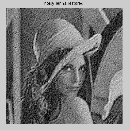
The MSE for the restored image is 1247.3. We see the same noise specs as we had seen with the inverse filter. But the image is in general better than the noisy image restored using the inverse filtering method and has a lower MSE. So we can conclude that the direct inverse filtering method is better for a noiseless case and the iterative method is better when noise is present.

Q3) Explain Butterworth in Image Processing

A3)

BUTTERWORTH

Set this keyword to the dimension of the Butterworth filter to apply to the frequency domain. With a Butterworth bandpass filter, frequencies at the center of the frequency band are unattenuated and frequencies at the edge of the band are attenuated by a fraction of the maximum value. The Butterworth filter does not have sharp discontinuities between frequencies that are passed and filtered.

The default for BANDPASS_FILTER is BUTTERWORTH=1.

The centered FFT is filtered by one of the following functions, where D0 is the center of the frequency band, W is the width of the frequency band, D=D(u,v) is the distance between a point (u,v) in the frequency domain and the center of the frequency rectangle, and n is the dimension of the Butterworth filter:

A low Butterworth dimension is close to Gaussian, and a high Butterworth dimension is close to Ideal.

Q4) Define Wiener Filtering

A4)

The inverse filtering is a restoration technique for deconvolution, i.e. when the image is blurred by a known lowpass filter, it is possible to recover the image by inverse filtering or generalized inverse filtering. However, the inverse filtering is very sensitive to additive noise. The approach of reducing one degradation at a time allows us to develop a restoration algorithm for each type of degradation and simply combine them. The Wiener filtering executes an optimal tradeoff between inverse filtering and noise smoothing. It removes the additive noise and inverts the blurring simultaneously.

The Wiener filtering is optimal in terms of the mean square error. In other words, it minimizes the overall mean square error in the process of inverse filtering and noise smoothing. The Wiener filtering is a linear estimation of the original image. The approach is based on a stochastic framework. The orthogonality principle implies that the Wiener filter in the Fourier domain can be expressed as follows:

Where are respectively power spectra of the original image and the additive noise, and is the blurring filter. It is easy to see that the Wiener filter has two separate parts, an inverse filtering part and a noise smoothing part. It not only performs the deconvolution by inverse filtering (highpass filtering) but also removes the noise with a compression operation (lowpass filtering).

Q5) Write an implementation of Wiener Filter

A5)

Implementation

To implement the Wiener filter in practice we have to estimate the power spectra of the original image and the additive noise. For white additive noise, the power spectrum is equal to the variance of the noise. To estimate the power spectrum of the original image many methods can be used. A direct estimate is the periodogram estimate of the power spectrum computed from the observation:

Where Y(k,l) is the DFT of the observation. The advantage of the estimate is that it can be implemented very easily without worrying about the singularity of the inverse filtering. Another estimate which leads to a cascade implementation of the inverse filtering and the noise smoothing is

Which is a straightforward result of the fact: The power spectrum can be estimated directly from the observation using the periodogram estimate. This estimate results in a cascade implementation of inverse filtering and noise smoothing:

The disadvantage of this implementation is that when the inverse filter is singular, we have to use the generalized inverse filtering. People also suggest the power spectrum of the original image can be estimated based on a model such as the model.

Q6) What is Wavelet-based Image Restoration?

A6)

Although the Wiener filtering is the optimal tradeoff of inverse filtering and noise smoothing, in the case when the blurring filter is singular, the Wiener filtering amplifies the noise. This suggests that a denoising step is needed to remove the amplified noise. Wavelet-based denoising scheme, a successful approach introduced recently by Donoho, provides a natural technique for this purpose. Therefore, the image restoration contains two separate steps: Fourier-domain inverse filtering and wavelet-domain image denoising. The diagram is shown as follows.

Donoho's approach for image restoration improves the performance, however, in the case when the blurring function is not invertible, the algorithm is not applicable. Furthermore, since the two steps are separate, there is no control over the overall performance of the restoration. Recently, R. Neelamani et al. Proposed a wavelet-based deconvolution technique for ill-conditioned systems. The idea is simple: employ both Fourier-domain Wiener-like and wavelet-domain regularization. The regularized inverse filter is introduced by modifying the Wiener filter with a new-introduced parameter:

The parameter can be optimally selected to minimize the overall mean-square error. The diagram of the algorithm is displayed as follows.

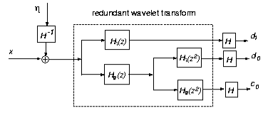
The implementation of the regularized inverse filter involves the estimation of the power spectrum of the original image in the spatial domain. Since wavelet transforms have good decorrelation property, the wavelet coefficients of the image can be better modeled in a stochastic model, and the power spectrum can be better estimated. This inspires a new approach: changing the order of the regularized inverse filtering and the wavelet transform. (See the following diagram)

This way both inverse filtering and noise smoothing can be performed in the wavelet domain. Specifically, the power spectrum of the image in the same subband can be estimated under the assumption that the wavelet coefficients are independent. Therefore, the power spectrum is just the variance of the wavelet coefficients. We note that the exchange of the order of inverse filtering and wavelet transform is valid only when undecimated wavelet transform is used and the blurring function is separable. Therefore, for interpretation, we can exchange the order of the blurring operation and the wavelet transform, which means that the inverse filtering cancels the blurring in the wavelet domain. So, wavelet thresholding results in a reasonable estimate. The above explanation can be visualized using the following figure.

Q7) Explain Notch filters in details with example

A7)

• Are used to remove repetitive "Spectral" noise from an image
• Are like a narrow highpass filter, but they "notch" out frequencies other than the dc component
• Attenuate a selected frequency (and some of its neighbors) and leave other frequencies of the Fourier to transform relatively unchanged

Repetitive noise in an image is sometimes seen as a bright peak somewhere other than the origin. You can suppress such noise effectively by carefully erasing the peaks. One way to do this is to use a notch filter to simply remove that frequency from the picture. This technique is very common in sound signal processing where it is used to remove mechanical or electronic hum, such as the 60Hz hum from AC power. Although it is possible to create notch filters for common noise patterns, in general notch filtering is an ad hoc procedure requiring a human expert to determine what frequencies need to be removed to clean up the signal.

The following is an example of removing synthetic spectral "noise" from an image.

Noisy Image	Fourier Spectrum of Image (noise peaks circled)
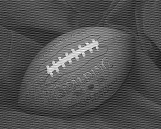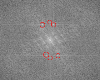Image after Butterworth notch filters	The spectrum of the image after Butterworth notch filters

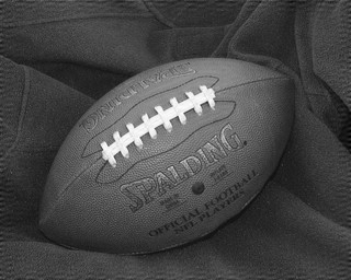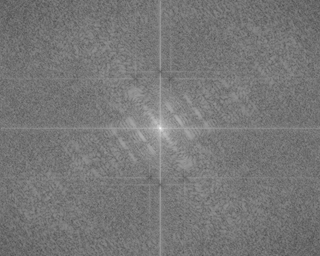The above images were created using four M-files(paddedsize.m, lpfilter.m, dftuv.m, and notch.m), noiseball.png, and the following MATLAB calls

FootBall=imread('noiseball.png');

Imshow(footBall)

%Determine good padding for Fourier transform

PQ = paddedsize(size(footBall));

%Create Notch filters corresponding to extra peaks in the Fourier transform

H1 = notch('btw', PQ(1), PQ(2), 10, 50, 100);

H2 = notch('btw', PQ(1), PQ(2), 10, 1, 400);

H3 = notch('btw', PQ(1), PQ(2), 10, 620, 100);

H4 = notch('btw', PQ(1), PQ(2), 10, 22, 414);

H5 = notch('btw', PQ(1), PQ(2), 10, 592, 414);

H6 = notch('btw', PQ(1), PQ(2), 10, 1, 114);

% Calculate the discrete Fourier transform of the image

F=fft2(double(footBall),PQ(1),PQ(2));

% Apply the notch filters to the Fourier spectrum of the image

FS_football = F.*H1.*H2.*H3.*H4.*H5.*H6;

% convert the result to the spatial domain.

F_football=real(ifft2(FS_football));

% Crop the image to undo padding

F_football=F_football(1:size(footBall,1), 1:size(footBall,2));

%Display the blurred image

Figure, imshow(F_football,[])

% Display the Fourier Spectrum

% Move the origin of the transform to the center of the frequency rectangle.

Fc=fftshift(F);

Fcf=fftshift(FS_football);

% use abs to compute the magnitude and use log to brighten display

S1=log(1+abs(Fc));

S2=log(1+abs(Fcf));

Figure, imshow(S1,[])

Figure, imshow(S2,[])

Q8) Explain Optimum Notch Filtering

A8)

When several interference components are present or if the interference has broad skirts a simply notch filter may remove too much image information.

One solution is to use an optimum filter that minimizes local variances of the restored estimate.

Such “smoothness” constraints are often found in optimum filter design

1. Manually place a notch pass filter HNP at each noise spike in the frequency domain. The Fourier transform of the interference noise pattern is

2. Determine the noise pattern in the spatial domain

3. Conventional thinking would be to simply eliminate noise by subtracting the periodic noise from the noisy image

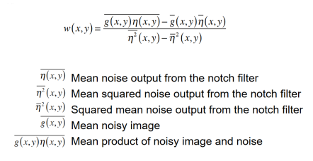
4. To construct an optimal filter consider

Where w(x,y) is a weighting function.

5. We use the weighting function w(x,y) to minimize the variance 2(x,y) with respect to w(x,y)

We only need to compute this for one point in each non-overlapping neighborhood.

Q9) Explain BLIND DECONVOLUTION in detail 

A9)

Many different methods were attempted to restore our image when we don't explicitly know h. Most of them had very little success. The reasons will be explained as we explain the general approach we used. The methods for estimating h are known as Blind Deconvolution because our inverse filtering (deconvolution) is being performed without knowledge of our blurring function. The methods we used were all homomorphic ideas.

In general, our degradation is modeled as a convolution plus noise. In the frequency domain, convolution becomes multiplication. If we ignore the additive noise, we can take the log of the multiplication and get addition. Thus, the log of the FT of our degraded image DI is equal to the log of the FT of the original image OI plus the log of the Transfer Function H. Now that we have added, we can use statistical estimation to estimate H and thus solve for OI.

The problem with this method is that in practice we can't ignore the noise. Therefore, we need ways to estimate the log of the multiplication of OI and H plus the Noise Spectrum. The first approach we had success with came from the Jain text. It uses the following estimate for H.

Uk and Vk are obtained by breaking the input image (u) and degraded image (v) into M smaller blocks and computing their Fourier Transforms. H is then used with Snn and Suu to compute the Wiener Filter. Notice that this method only computes the Magnitude of H, so it's best for phaseless LSI filters. This necessitated our filter design of a phaseless h. The following pictures show the Magnitude Plots of the actual and estimated transfer functions. Our image degradation model is the same as always, and we calculated H using the above equation with M = 16. This broke down the images into 64x64 pixel blocks.

Magnitude Plot of Blurring Filter	Magnitude Plot of Estimated Blurring Filter

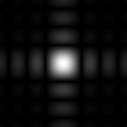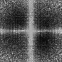Note that we capture the form of the degradation filter, but we have a lot more noise. Surprisingly, our restoration MSE isn't too bad, depicted below. With noise variance 80. Also, since we are restoring using Wiener Filtering, we estimate Snn and Suu for restoration.

Lenna after Blurring Plus Noise	Lenna restored using Jain Approach
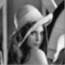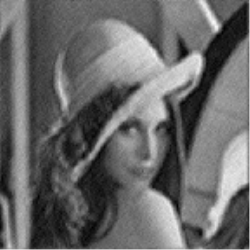Mean Squared Error = 1.0660e+05	Mean Squared Error = 283.1

We see that our MSE has gone from 256 with unknown Snn to 283 with all three Wiener Filter components (h, Suu, * Snn). We can see that some of the blurrings have been reduced in our restored image. Lines can be seen in the band around the hat and the boa is a bit clearer. However, even though our MSE isn't too bad, this is the worst image restoration thus far with respect to visual aspects. Most of the restoration was magnitude restoration. But this was by far our greatest success at blind deconvolution.

Our second approach came from the Lim text. It was proposed by Stockham. The homomorphic idea of taking the log in the frequency domain is again present, as is the notion of breaking up the picture into M sub-blocks. The equation estimates the denominator of the PSE filter as follows:

Where C is Euler's constant (0.57221...). Note that H is never calculated directly. Instead, we use this estimation to choose our PSE filter and restore our image. Our attempt at restoration with this method is shown below. Again, the variance is 80, but Suu and Snn are assumed known. Recall that if Snn is not explicitly known, then our PSE restoration fails.

Lenna after Blurring Plus Noise	Lenna restored using Stockham Approach
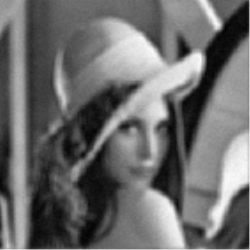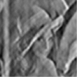Mean Squared Error = 1.0656e+05	Mean Squared Error = 7.4031e+07

Clearly, our restoration has further degraded our image. This was seen earlier when we attempted PSE restoration without knowledge of Snn. In this case, we are trying to estimate the entire denominator, not just Snn. Our restoration suffers greatly.

We conclude that Power Spectrum Equalization is just a poor restoration choice in general. It fails for unknown Snn and for our attempt at unknown h. The lack of inverse filtering makes the denominator extremely important in restoration, so no estimation will be very robust. Supposedly, there are cases where PSE is preferable to Wiener Filtering [Castleman], but our models do not fit them.

There are direct methods for blind deconvolution as well, but we attempted only indirect methods because they are less ad hoc. An example of a direct method for blind deconvolution is to model lines normal to a suspected edge in the degraded image as the integral of h and use this measurement for deconvolution. Another indirect method we tried was to assume there was no additive noise in the system. Thus, if our average blurring function goes to zero over many images, we can estimate our original frequency information as the geometric mean of the degraded images. However, geometric means are extremely vulnerable to noise, and many iterations were required for our approximations to hold. In general, we did not get good results for this method.