UNIT-5

Speech Analysis

Q1) Write in short about Feature Extraction and the techniques used for it.

A1) Features of a speech signal

When we are in contact with a speech signal, we learn a lot about it which makes it very easy to perform different tasks with. There are several methods that can be used in order to determine the different features used in a feature signal. We can broadly classify the same into 2 parts.

There are two types of features of a speech signal:

• The temporal features (time domain features) : These are the features that are straightforward in order to track the simple interpretations like the energy if a signal as well as the crossing rate which can amplify he amplitude.
• The spectral features (frequency - based features) : These are the features that are primarily based by obtaining the changing signals in the domain which is related to frequency. We can exploit the model the elements with the mass of the central tendency. The options can be used in order to establish the pitch and rhythm of the sound.

Feature Extraction & Pattern Comparison Techniques

Speech process may be performed at completely different 3 levels. Amplitude process considers the anatomy of human sensory system and method signal in kind of little chunks known as frames. In sound level process, speech phonemes are noninheritable and processed.

Phoneme is that the basic unit of speech. Third level process is thought as word level process. This model concentrates on linguistic entity of speech. The Hidden Markov Model (HMM) may be accustomed represent the acoustic state transition within the word.

The notes are organized as follows: Section a pair of describes acoustic feature extraction. In section three, details of the feature extraction techniques like LPC, PLP and MFCC are mentioned.

Q2) What are the different types of coefficients? Write in detail about each one.

A2) There are 3 types of coefficients namely

1.      Mel Frequency Cepstrum Coefficients (MFCC)

The rifest and dominant methodology accustomed extract spectral options is scheming Mel-Frequency Cepstral Coefficients (MFCC). MFCCs are one in every of the foremost fashionable feature extraction techniques utilized in speech recognition supported frequency domain exploitation the Mel scale that relies on the human ear scale. MFCCs being thought of as frequency domain options are rather more correct than time domain options.

Mel-Frequency Cepstral Coefficients (MFCC) may be an illustration of the $64000 cepstral of a windowed short signalling derived from the quick Fourier remodel (FFT) of that signal. The distinction from the $64000 cepstral is that a nonlinear frequency scale is employed, that approximates the behaviour of the sensory system. To boot, these coefficients are strong and reliable to variations per speakers and recording conditions. MFCC is associate audio feature extraction technique that extracts parameters from the speech almost like ones that are employed by humans for hearing speech, whereas at an equivalent time, deemphasizes all alternative info. The speech signal is initial divided into time frames consisting of associate impulsive range of samples. In most systems overlapping of the frames is employed to swish transition from frame to border. Every time frame is then windowed with playacting window to eliminate discontinuities at the sides. The formula for the various coefficients are as follows :

Where N is total range of sample and n is current sample. Once the windowing, quick Fourier Transformation (FFT) is calculated for every frame to extract frequency elements of an indication within the time domain. FFT is employed to hurry up the process.

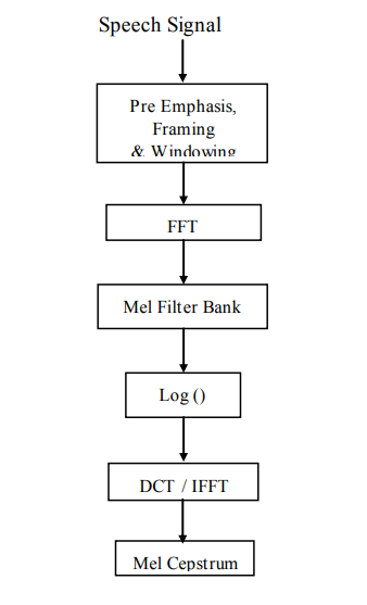Fig. Description 1: The above representation is of the derivation through the MFCC method

Linear Predictive Coding (LPC)

It is fascinating to compress signal for economical transmission and storage. Digital signal is compressed before transmission for economical utilization of channels on wireless media. For medium or low bit rate applied scientist, LPC is most generally used [13]. The LPC calculates an influence spectrum of the signal. It's used for formant analysis [14]. LPC is one in every of the foremost powerful speech analysis techniques and it's gained quality as a formant estimation technique [15].

While we have a tendency to pass the speech signal from speech analysis filter to get rid of the redundancy in signal, residual error is generated as associate output. It are often amount by smaller variety of bits compare to original signal. So now, rather than transferring entire signal we will transfer this residual error and speech parameters to get the initial signal. A constant model is computed supported least mean square error theory; this method being referred to as linear prediction (LP). By this technique, the speech signal is approximated as a linear combination of its p previous samples

In this technique, the obtained LPC coefficients describe the formants. The frequencies at that the resonant peaks occur area unit known as the formant frequencies [16]. Thus, with this technique, the locations of the formants in an exceedingly speech signal area unit calculable by computing the linear prophetic coefficients over a window and finding the peaks within the spectrum of the ensuing LP filter. We've got excluded 0th constant and used next 10 LPC Coefficients.

In speech generation, throughout speech sound vocal cords vibrate harmonically and then similar periodic signals area unit created. Whereas just in case of consonant, excitation supply is often thought of as random noise [17]. Vocal tract works as a filter, that is to blame for speech response. Biological development of speech generation is often simply born-again in to equivalent mechanical model. Periodic impulse train and random noise are often thought of as excitation supply and digital filter as vocal tract.

Perpetual Linear Prediction (PLP)

The sensory activity Linear Prediction PLP model developed by Hermansky. PLP models the human speech supported the conception of hearing [2, 9]. PLP discards extraneous info of the speech and so improves speech recognition rate. PLP is just like LPC except that its spectral characteristics are reworked to match characteristics of human sensory system.

Fig. Description 2: The above diagram is the block representation of the PLP method

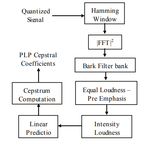
Fig. Description 3: The parameters involved in the PLP computation are mentioned in the above diagram.

The 3 steps frequency warp, smoothing and sampling area unit integrated into one filter-bank known as Bark filter bank. Associate equal loudness pre-emphasis weight the filter-bank outputs to simulate the sensitivity of hearing. The equal values area unit reworked in line with the facility law of Stevens by raising every to the facility of zero.33. The ensuing sensory system crooked spectrum is more processed by linear prediction (LP). Applying LP to the sensory system crooked spectrum means we have a tendency to cypher the predictor coefficients of a (hypothetical) signal that has this crooked spectrum as an influence spectrum. Finally, Cepstral coefficients area unit obtained from the predictor coefficients by a formula that's like the log of the model spectrum followed by associate inverse Fourier rework.

Q3) What are speech distortion measures? Name the 2 considerations used for the same.

A3) Speech Distortion Measures

When we are trying to detect the different types of speech that we come in contact with we need to understand the whole process which can be understood with the help of the diagram that is given below:

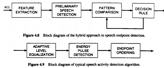
Fig. Description 4 : This is the comparison between the hybrid and the normal (typical) methods used to approach speech detection.

Mathematical Considerations

When we have a look at the different patterns that can be part of the entire process of finding algorithms, we can see distortion. The main component that is part of the algorithms that are used in order to compare speech patterns, is the dissimilarity between each of the sustained speeches. To allow us to gain some kind of better understanding of the above we have 3 separate rules which are used.

Let us assume that there are 2 vectors which are feature vectors in nature. Let us call them x and y. These function on a distance function which is represented as d on a vector space that is represented as X.

1. 0 d(x,y) < infinity if x,y belong to vector space X

This property is also known as positive definiteness

2.     d(x,y) = 0 if x = y

3.     d(x,y) = d(y, x) if x,y belong to vector space X

This is known as symmetry condition

4.     d(x,y) ≤ d(x, z) + d(y, z) if x, y, z belong to vector space X

This is known as triangle inequality condition

If we have the distance d that satisfies any of the property, we call it a distortion measure. It is very difficult to house separate objectives that are dual in nature to the meaning as well as the mathematical significance of the same.

Perceptual Considerations

When we are in need of deciding a certain factor that is key in order to choose an appropriate name as well as concept for the judgement, we see a certain relevance that is entirely phonetic. We are able to compare the bandwidth to the frequency with the help of the following figures. We are able to see the distribution of perturbations across the bandwidth and get an idea of the dissimilarities that are present between the voice signals.

The intensity of the bandwidth is given by a formula which is worked out as given below:

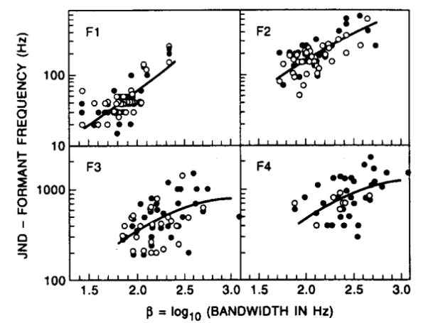Fig. Description 5: This gives us a graphical visual at the LPC pole frequencies as a function of the bandwidths. The darker circles are a sign of perturbations that are positive in nature. There are also circles with only an outline that represent the perturbations that are negative in nature.

Q4) Write about log spectral distances and Cepstral Distances.

A4) Log Spectral Distances

If we consider two spectra which are represented as S(w) and S’(w) respectively, we would have the difference between the magnitude exhibited by each given by the formula

                                             V( w ) = log S( w ) – log S’( w )

Once we get an idea about the different measures that surround the log spectral distance we get an idea about the same in terms of graphical structures as represented below.

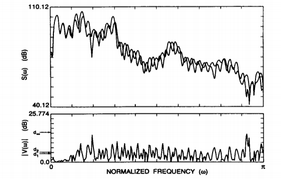Fig. Description 6 : The above representation is of two power spectra that are ambiguous to the S(w) in terms of the logarithmic scale and the function V(w) as given above.

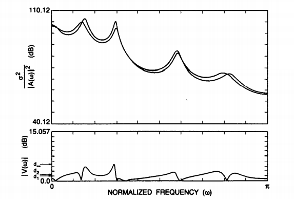Fig. Description 7 : This is the representation of an LPC model which is in correspondence to the spectra S(w) and the function V(w) as given above.

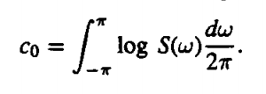
Cepstral Distances

When we need to understand about the next type of distance in question we need to understand the Fourier transform of the logarithm of the signal which is in the context. To understand the spectrum hat is related to the power we need to allow it to undergo a Fourier transformation which allows it to be symmetric with respect to w = 0 (omega). The expression can be depicted as shown below:

The coefficients are known as cepstral coefficients and are given by the formula:

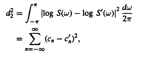
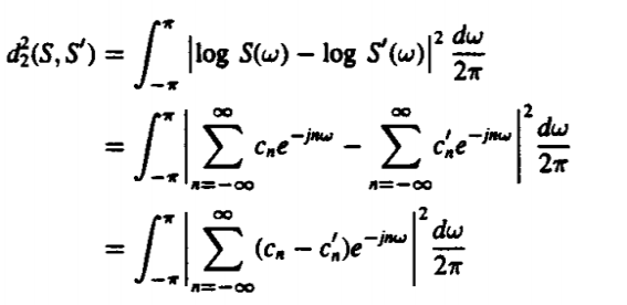
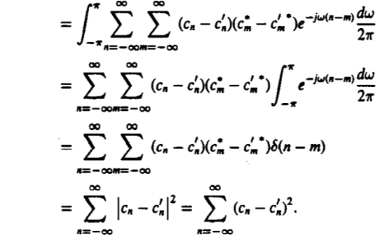
Finally, if we want to compare the two spectra that we have taken viz. S(w) and S’(w) we can do so by using Parseval’s theorem. The formula is essentially the Root Mean-Squared of the logarithm in the theorem.

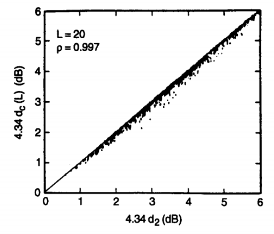
However, at times we realise that the Cestrum is essentially a sequence that is going to decay further. This is because it does not receive an infinite number of terms back. This is why the process of LPC models that are smoothed to a very large extent have their terms truncated. This gives rise to a new term which is also known as truncated cepstral distance. It is given by the formula.

Fig. Description 8 : We can see a clear indication of the scatter plot that tells us about the comparison between a regular cepstral distance and a truncated cepstral distance. This is carried out for 800 pairs of models. The truncation is only done till there are 20 terms.

Q5) Prove

A5)

Q6) Write in brief about spectral distortion using a warped frequency scale and likelihood distortions

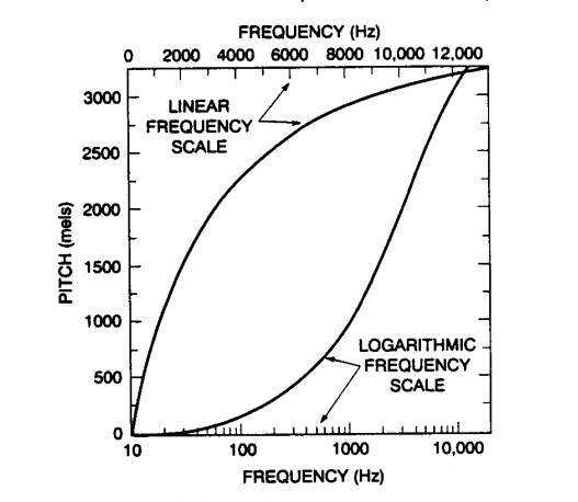
A6) After a lot of research that has been done in the field of sound it is for certain that the speech signals that humans use to converse are not in tune with a linear scale. In order to find better tones and pitches that can sound realistic as well as give an idea about the true matching, a warped scale was designed.

Fig. Description 10: Here we can see a clear comparison between a frequency scale that is linear as well as one that has been tuned to be in the form of a logarithmic scale.

The property that goes with an LP model while it makes approximations about frequencies is that it makes all of them equally. However, it is noticed that the human auditory senses have a resolution that is directly proportional to the frequency. This is the reason why a warped model has been prepared that can allow the frequencies in the lower range to have more area. This allows it to be functional even when the order goes below a certain level in the human auditory range.

This type of distortion is raised in a manner very similar to how the equation for V(w) was obtained. We can find that the linear predictive model uses the maximum likelihood model in order to find out the equations as given below:

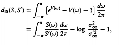The outcomes in terms of infinities are simply prediction errors for the spectra S(w) and S’(w). We are able to use this spectrum in order to measure the properties that might show some type of similarities in nature. We find the equation replacing the spectrum S’(w) with the path order of a spectrum as shown below :

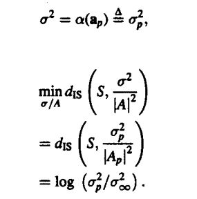
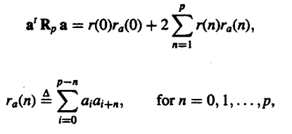
We can further simplify the distortion in the equation as follows. This will be followed by rewriting the energy which is left in the terms of a summation series :

We get to see another case in which the spectrum is replaced by a different pole model. This is given as follows:

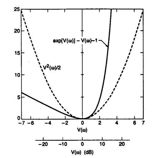Fig. Description 9: This is the comparison which is done between both the two integrals that were formed as a result of the spectrum S(w) being replaced by another pole spectrum model

Q7) Write a short note about Time Alignment and Normalization?

A7) This sub section consists of different restraints in the section. Linear normalization essentially makes the assumption that the rate of speaking is always proportional to the rate of utterance. We can see this in the diagram that is given below to get a better idea of the same.

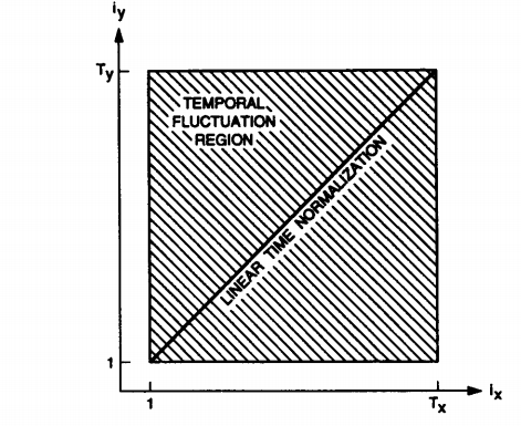Fig. Description 11: We can see the comparison and alignment between two very different sequences which also have different durations.

In order to have the process of normalization complete there need to be certain constraints that are put through in the entire process. There are some which are very meaningful while some which are just different from one another. This causes a lot of problems if not sorted out. There are various types of constraints which are given below.

• Constraints of the endpoint

There are different end points which are used to mark the culmination and termination of a certain corpus. The endpoint is obtained by using the information which is received from the operation that is used to detect speech.

• Constraints regarding monotonicity

There is a need to bring order while normalization. This is why the constraints of monotonicity are used to maintain order that is temporal. The constraint simply means that any path that is being evaluated will not have a slope of negative value.

• Constraints regarding the local continuity

Warping may cause the temporal matchings a lot of problem in terms of the continuity. There may be different omissions that could leave space between each of the element. This is bound to give inaccurate results. These constraints are used in order to make sure that the continuity is checked at regular intervals.

We are also able to get an idea about the different types on constraints in terms of the path that is followed by each of them. The diagram as well as notation of each of them is given below:

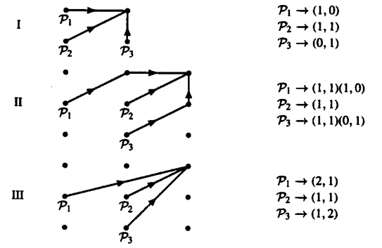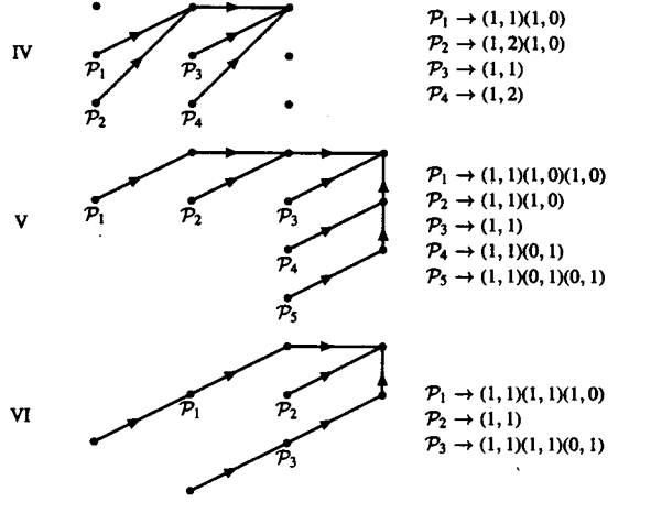
• Constraints regarding the global path

In the bargain of taking care of all the different local continuations there might be some problems in terms of the entire overlook. This is why there are certain constraints that are made to exclude certain portions in order to have a warping system that is optimal in nature. In the equation given below, l represents the index of the path that is allowed. Pl represents the path that is allowed and Tl represents the total moves that can be carried out in order to reach the final position.

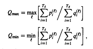• The weighing of the slope

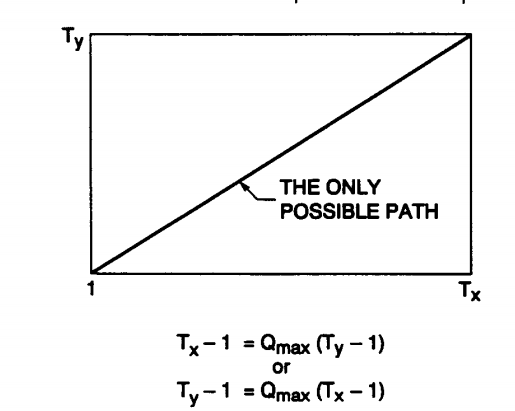
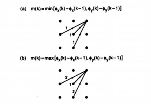
This is another method which is used in order to achieve warping that is very optimal in nature. This adds a new dimension to the entire sequence. The function m(k) is used in order to control the function on a higher scale.

Fig. Description 12: This is the representation of the extreme cases that allow only warping in terms of a path that is linear in nature. Some of the equations in terms of m(k) are given below.

Q8) What is Dynamic Time Warping ?

A8) Dynamic Time Warping

Dynamic time warping is a part of the Normalization process because it takes the help of various constraints that are used in order to work out the optimal warping process. This can be understood better by look at some of the paths and constraints that are used in order to follow up with the normalization process.

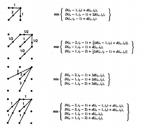Fig. Description 13: This talks about the different paths taken which can help find the best and optimal warping path.

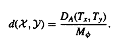
There are 3 steps which go into the process to ensure that the programming has a recursion process that is independent of the path used for warping. This tells us the most optimal path to get from a point (1,1) to the point (Tx , Ty).

• Initialization

• Recursion

• Termination

Q9) Write about the Multiple time alignment path. (Parallel Algorithm)

A9) Multiple Time – Alignment Path

The main feature that one would use in order to understand the principle of optimality is an algorithm. Getting the work done in the least number of steps is the main aim of the algorithms. We can find the k-best paths through the process of optimizing our search. To find the best path we need to take into account all of the existing N paths. The points that are associated with them as well as their connections are very important to have. We can understand a little more about these process with the help of an algorithm that is used for the process:

• Parallel Algorithm

This algorithm states that the path which is second best after a certain M^th move could reach the same point as the best path that could be chosen. We could use this information to find the second-best path after the M number of moves. This algorithm makes use of a method which is parallel to the best path which is where it gets its name from. Using the kth small value, we can find the value of n1 and n2 as given below:

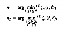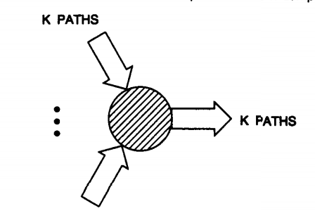Fig. Description 14: This is the visual representation of finding the k paths that are best through the parallel algorithm.

As we move forward in the path it is very obvious that the relation become recursive. We need to keep noting the values after proper examination. This would help us gain and idea of every move before selecting the proper move to branch out from. Hence we finally obtain

Q10) What is Baum Welch Re-estimation? Explain.

A10) Baum – Welch Re-Estimation

In order to understand and comprehend the HMM models we need to understand what the parameters might be. In order to help us with this we use an algorithm which is known as the Baum – Welch Re-Estimation Algorithm. We can simply see a mixture that is represented below (Gaussian). This would have to be sorted in order to get it in place to run through the algorithm.

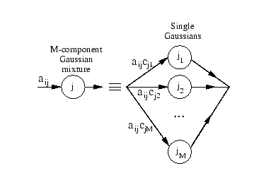Fig. Description 15: The following is a Gaussian Mixture that is being separated similar to the operation going to take place in the algorithm.

We need to make an estimate about the mean and variance of the data that is going to be used in the HMM model. The Gaussian components are very important and need to be used to get the best idea about the data coming through. If we needed to find the averages in a single phase we would use the formulas given below.

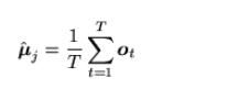However, the real models are bound to have multiple states that are used in practicality. Using the likelihood and assigning vectors to the parameters we could obtain a better result. If there is a probability density of all the multiple states, we could modify the formulas given above to the following.

We could further write about the different steps that are used in the algorithm as follows :

• Re-Estimation needs to occur in order to allocate a certain amount of storage for the numerator as well as the denominator that appears in each and every equation.
• The probabilities (both forward and backward) need to be calculated for all the different states.
• The accumulators of the state need to be based on the observation through the vector value.
• These values need to be used in order to calculate the parameter values (new).
• If the value is not higher than the previous iteration that means we have reached the endpoint. However, if the value is still higher, continue the iterations to get the desired new parameter values.

Q11) Write in short about the Viterbi Search Algorithm.

A11) Viterbi Search

For a model that is in use like HMM it is important to note that there are numerous variables that are hidden in nature. One needs to find these variables and work on the sequence of the same. This is the decoding part of the job. It is made up of 3 parts that we can see easily.

• Initialization

• Recursion

• Termination

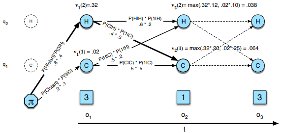Fig. Description 16 : This tells us about the best paths that can be used in order to compute the hidden state sequences which are used in the process of HMM.

Implementation Issues

1. HMM models have a problem due to the label bias problem. Once the state has been selected, the observation which is going to succeed the current one will select all of the transitions that might be leaving the state.

2.     There are a few examples in words such as “rib” and “rob” which when placed in the algorithm in their raw from have a little different path as compared to the other words. When we have “r_b” there is a path that goes through 0-1 and 0-4 to get the probability mass function.

3.     Both the paths would be equally likely not allowing the model to select one fixed word that could be predicted by the model correctly. HMM models are used to tag and have their own pros and cons which can be decided based on the model that needs to be adapted.