undefined | unit 5 trees and graph

Back to Study material

Data Structure & Algorithm

MODULE 5

Trees and Graph

Explain the basic tree terminologies?

A tree is defined as a set of one or more nodes T such that:

There is a specially designed node called root node

The remaining nodes are partitioned into N disjoint set of nodes T1, T2,…..Tn, each of which is a tree.

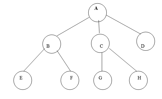
Fig. 4.1 Example of tree

In above tree A is Root.

Remaining nodes are partitioned into three disjoint sets:

{B, E, F}, {C, G, H}, {D}.

All these sets satisfies the properties of tree.

Some examples of TREE and NOT TREE

Each linear list is trivially a tree

Not a tree: cycle A→A

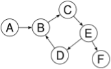
Not a tree: cycle B→C→E→D→B

Not a tree: two non-(connected parts, A→B and C→D→E

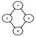
Not a tree: undirected cycle 1-2-4-3

Fig. Examples of tree and no tree

Tree Terminologies

Root – The top node in a tree.

Parent – The converse notion of child.

Siblings – Nodes with the same parent.

Descendant – a node reachable by repeated proceeding from parent to child.

Ancestor – a node reachable by repeated proceeding from child to parent.

Leaf – a node with no children.

Internal node – a node with at least one child.

External node – a node with no children.

Degree – number of sub trees of a node.

Edge – connection between one node to another.

Path – a sequence of nodes and edges connecting a node with a descendant.

Level – The level of a node is defined by 1 + the number of connections between the node and the root.

Height of tree –The height of a tree is the number of edges on the longest downward path between the root and a leaf.

Height of node –The height of a node is the number of edges on the longest downward path between that node and a leaf.

Depth –The depth of a node is the number of edges from the node to the tree's root node.

Forest – A forest is a set of n ≥ 0 disjoint trees.

2. Explain the different types of trees?

Binary Tree

A binary tree is a special cas eof tree in which no node of a tree can have degree more than two.

Definition of Binary Tree:

A binary tree is made of nodes, where each node contains a "left" pointer, a "right" pointer, and a data element. The "root" pointer points to the topmost node in the tree. The left and right pointers recursively point to smaller "subtrees" on either side. A null pointer represents a binary tree with no elements -- the empty tree.

The formal recursive definition is A binary tree is either empty (represented by a null pointer), or is made of a single node, where the left and right pointers (recursive definition ahead) each point to a binary tree.

Example of Binary Tree:

Fig.Example of Binary Tree

Types of Binary Tree,

1. Left Skewed Binary Tree:

2. Right Skewed Binary Tree:

1. Left Skewed Binary Tree:

Fig. 4.6 Example of Left Skewed Binary Tree

In this tree, every node is having only Left sub tree.

3. Right Skewed Binary Tree:

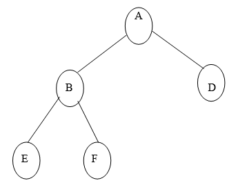
Fig. Example of Right Skewed Binary Tree

In this tree, every node is having only Right sub tree.

Full or strict Binary Tree:

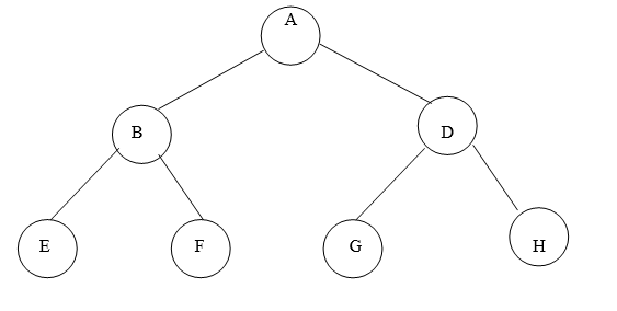
It is a binary tree of depth K having 2k-1 nodes.

For k=3, number of nodes=7

$F:\work\AKU\CSE\SEM 3 NEW\DATA STRUCTURE\Untitled.png$

Fig. Example of strict Binary Tree

Complete Binary Tree:

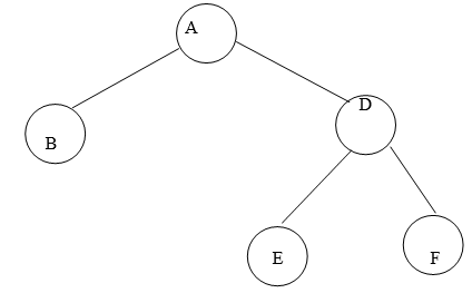
It is a binary tree of depth K with N nodes in which these N nodes can be numbered sequentially from 1 to N.

Since a binary tree is an ordered tree and has levels, it is convenient to assign a number to each node.

Suppose for K=3:

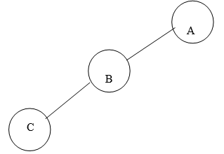
Fig. Example of Complete Binary Tree

The nodes can be numbered sequentially like:

Node number	Node
1	A
2	B
3	D
4	E
5	F

Fig. Representation of Complete Binary Tree

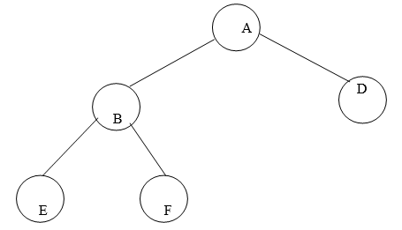
Consider another example of binary tree:

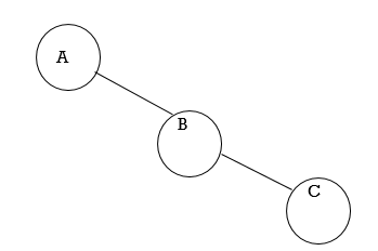
Fig. 4.11 Example of Non Complete Binary Tree

If we try to give numbers to nodes it would appear like:

Node number	Node
1	A
2	B
3	D
4	-
5	-
6	E
7	F

Fig. 4.12 Representation of Non Complete Binary Tree

Here nodes cannot be numbers sequentially, so this kind of tree cannot be called as a complete binary tree

Binary Search Tree

We now turn our attention to search tress: Binary Search tress in this chapter and AVL Trees in next chapter. As seen in previous chapter, the array structure provides a very efficient search algorithm, the binary search, but it is inefficient for insertion and deletion algorithms. On the other hand, linked list structure provides efficient insertion and deletion algorithms but it is very inefficient for search algorithm. So what we need is a structure that provides efficient insertion, deletion as well as search algorithms.

4. Explain binary threaded tree?

"A binary tree is threaded by making all right child pointers that would normally be null point to the inorder successor of the node (if it exists), and all left child pointers that would normally be null point to the inorder predecessor of the node."

It is also possible to discover the parent of a node from a threaded binary tree, without explicit use of parent pointers or a stack. This can be useful where stack space is limited, or where a stack of parent pointers is unavailable (for finding the parent pointer via DFS).

Inorder Threaded Binary Tree:

In inorder threaded binary tree, left thread points to the predecessor and right thread points to the successor.

Types Inorder Threaded Binary Tree:

Right Inorder Threaded Binary Tree.

In this type of TBT, only right threads are shown which points to the successor.

Left Inorder Threaded Binary Tree.

In this type of TBT, only left threads are shown which points to the predecessor.

For TBT it is not necessary that the tree must be BST, it can be applied to general tree.

5. Explain AVL trees

The concept is developed by three persons: Adelsion, Velski and Landis.

Balance Factor:

Balance factor is (Height of left sub tree - Height of right sub tree)

Height Balance Tree:

An empty tree is height balanced. If T is non empty binary tree with TL and TR as left and right sub tress, then T is height balanced if and only if:

TL and TR are height balanced.

HL- HR =1

HL and HR are heights of left and right sub tree.

For ant node in AVL tree Balance factor must be -1 or 0 or 1.

Following rotations are performed on AVL tree if any of the nodes is unbalanced.

1. LL Rotation.

2. LR Rotation.

3. RL Rotation.

4. RR Rotation.

1. LL Rotation:

Count from unbalanced node. First left node becomes the root node.

2. LR Rotation:

Count from unbalanced node. Go for left node and then right node say X. The node X becomes the root node.

3. RL Rotation:

Count from unbalanced node. Go for right node and then left node say X. The node X becomes the root node.

4. RR Rotation:

Count from unbalanced node. First right node becomes the root node.

While inserting data in AVL tree, Follow the property of Binary search tree (left<root<right)

6. Obtain an AVL tree by inserting one integer at a time in following sequence:

150,155,160,115,110,140,120,145,130

SOLUTION:

Step 1: insert 150

150

Balance factor for 150 is: 0 – 0=0

1500

NO ROTATION IS REQUIRED.

Step 2: insert 155

150-1

1550

Balance factor for 150 is: 0 – 1= -1

Both nodes are balanced.

NO ROATION IS REQIURED.

STEP 3: INSERT 160.

150-2

155-1

1600

Balance factor of 150 is -2. So 150 is unbalanced. Some rotation is required to do 150 as balanced node. Start from 150 towards 160.

150-2 R

155-1 R

1600

We get RR direction. So we have to perform RR rotation.

In RR rotation, Count from unbalanced node. First right node becomes the root node. So here first R is 155. So 155 will become the root.

1550

1500 1600

Now all nodes are balanced.

STEP 4: INSERT 115.

1551

1501 1600

1150

All nodes are balanced. NO ROTATION IS REQUIRED.

STEP 5: INSERT 110

1552

1502 1600

1151

1100

155 and 150 are unbalanced. Whenever two/more nodes are unbalanced, we have to consider the lowermost node first. i.e.150. move from 150 towards the node causing unbalancing (110)

1552

L 1502 1600

L 1151

1100

So we have to perform LL Rotation. In LL rotation, Count from unbalanced node. First Left node becomes the root node. So here first L is 115. So 115 will become the root.

1551

1150 1600

1100 1500

Now all nodes are balanced.

STEP 6: INSERT 140 1552

115-1 1600

1100 1501

1400

155 is unbalanced. Count move from 155 towards the node causing unbalancing (140).

1552

115-1 1600

1100 1501

1400

So we have to perform LR Rotation. In LR rotation, Count from unbalanced node(155). Go for left node and then right node (150). 150 will become root node

1500

1150 155-1

1100 1400 1600

Now all nodes are balanced.

STEP 7: INSERT 120

1501

115-1 155-1

1100 1401 1600

1200

Now all nodes are balanced.

STEP 7: INSERT 145

1501

115-1 155-1

1100 1400 1600

1200 1450

Now all nodes are balanced.

STEP 7: INSERT 130

1502

115-2 155-1

1100 1401 1600

120-1 1450

1300

Two nodes 150 and 115 are unbalanced. First consider 115. Count move from 115 towards the node causing unbalancing (130).

1502

115-2 155-1

1100 1401 1600

120-1 1450

1300

So we have to perform RL Rotation. In RL rotation, Count from unbalanced node(115). Go for Right node and then Left node (120). 120 will become root node.

1501

1200 155-1

1150 1400 1600

1100 1300 145

Now all nodes are balanced.

Thus the tree is balanced.

Searching: For searching element 1, we have to traverse all elements (in order 3, 2, 1). Therefore, searching in binary search tree has worst case complexity of O(n). In general, time complexity is O(h) where h is height of BST.

Insertion: For inserting element 0, it must be inserted as left child of 1. Therefore, we need to traverse all elements (in order 3, 2, 1) to insert 0 which has worst case complexity of O(n). In general, time complexity is O(h).

Deletion: For deletion of element 1, we have to traverse all elements to find 1 (in order 3, 2, 1). Therefore, deletion in binary tree has worst case complexity of O(n). In general, time complexity is O(h).

5.Explain the tree operations on each tree and their algorithm?

Following are the basic operations of a tree −

Search − Searches an element in a tree.

Insert − Inserts an element in a tree.

Pre-order Traversal − Traverses a tree in a pre-order manner.

In-order Traversal − Traverses a tree in an in-order manner.

Post-order Traversal − Traverses a tree in a post-order manner.

Node

Define a node having some data, references to its left and right child nodes.

struct node {

int data;

struct node *leftChild;

struct node *rightChild;

};

Search Operation

Whenever an element is to be searched, start searching from the root node. Then if the data is less than the key value, search for the element in the left subtree. Otherwise, search for the element in the right subtree. Follow the same algorithm for each node.

Algorithm

struct node* search(int data){

struct node *current = root;

printf("Visiting elements: ");

while(current->data != data){

if(current != NULL) {

printf("%d ",current->data);

//go to left tree

if(current->data > data){

current = current->leftChild;

} //else go to right tree

else {

current = current->rightChild;

}

//not found

if(current == NULL){

return NULL;

}

return current;

}

Insert Operation

Whenever an element is to be inserted, first locate its proper location. Start searching from the root node, then if the data is less than the key value, search for the empty location in the left subtree and insert the data. Otherwise, search for the empty location in the right subtree and insert the data.

Algorithm

void insert(int data) {

struct node *tempNode = (struct node*) malloc(sizeof(struct node));

struct node *current;

struct node *parent;

tempNode->data = data;

tempNode->leftChild = NULL;

tempNode->rightChild = NULL;

//if tree is empty

if(root == NULL) {

root = tempNode;

} else {

current = root;

parent = NULL;

while(1) {

parent = current;

//go to left of the tree

if(data < parent->data) {

current = current->leftChild;

//insert to the left

if(current == NULL) {

parent->leftChild = tempNode;

return;

}

} //go to right of the tree

else {

current = current->rightChild;

//insert to the right

if(current == NULL) {

parent->rightChild = tempNode;

return;

}

7. Explain the application of binary trees?

Huffman’s Algorithm:

Huffman Codes:

Huffman coding is a simple data compression scheme.

Fixed-Length Codes

Suppose we want to compress a 100,000-byte data file that we know contains only the lowercase letters A through F. Since we have only six distinct characters to encode, we can represent each one with three bits rather than the eight bits normally used to store characters:

Letter		A	B	C	D	E	F
Codeword	000		001	010	011	100	101

This fixed-length code gives us a compression ratio of 5/8 = 62.5%.

Variable-Length Codes

What if we knew the relative frequencies at which each letter occurred? It would be logical to assign shorter codes to the most frequent letters and save longer codes for the infrequent letters. For example, consider this code:

Letter	A	B	C	D	E	F
Frequency (K)	45	13	12	16	9	5
Codeword	0	101	100	111	1101	1100

Using this code, our file can be represented with

(45×1 + 13×3 + 12×3 + 16×3 + 9×4 + 5×4) × 1000 = 224 000 bits

or 28 000 bytes, which gives a compression ratio of 72%. In fact, this is an optimal character code for this file (which is not to say that the file is not further compressible by other means).

Prefix Codes

Notice that in our variable-length code, no codeword is a prefix of any other codeword. For example, we have a codeword 0, so no other codeword starts with 0. And both of our four-bit code words start with 110, which is not a codeword. Such codes are called prefix codes. Prefix codes are useful because they make a stream of bits unambiguous; we simply can accumulate bits from a stream until we have completed a codeword. (Notice that encoding is simple regardless of whether our code is a prefix code: we just build a dictionary of letters to code words, look up each letter we're trying to encode, and append the code words to an output stream.) In turns out that prefix codes always can be used to achieve the optimal compression for a character code, so we're not losing anything by restricting ourselves to this type of character code.

When we're decoding a stream of bits using a prefix code, what data structure might we want to use to help us determine whether we've read a whole codeword yet?

One convenient representation is to use a binary tree with the code words stored in the leaves so that the bits determine the path to the leaf. In our example, the codeword 1100 is found by starting at the root, moving down the right sub tree twice and the left sub tree twice.

Huffman’s algorithm is used to build such type of binary tree.

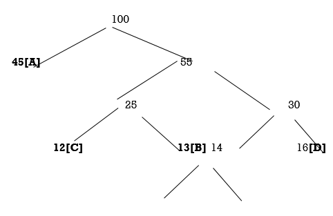
8. Find the Huffman algorithm for the following data :

Letter	A	B	C	D	E	F
Frequency (K)	45	13	12	16	9	5

Step1: sort the list in ascending order

5 9 12 13 16 45

Step2: New node’s frequency=5+9=14

12 13 14 16 45

Step3: New node’s frequency=12+13=25

14 16 25 45

Step4: New node’s frequency=14+16=30

25 30 45

Step4: New node’s frequency=25+30=55

45 55

Step4: New node’s frequency=45+55=100

100

Final Huffman’s tree will be:

9. Explain B+ tree?

Most queries can be executed more quickly if the values are stored in order. But it's not practical to hope to store all the rows in the table one after another, in sorted order, because this requires rewriting the entire table with each insertion or deletion of a row.

This leads us to instead imagine storing our rows in a tree structure. Our first instinct would be a balanced binary search tree like a red-black tree, but this really doesn't make much sense for a database since it is stored on disk. You see, disks work by reading and writing whole blocks of data at once — typically 512 bytes or four kilobytes. A node of a binary search tree uses a small fraction of that, so it makes sense to look for a structure that fits more neatly into a disk block.

Hence the B+-tree, in which each node stores up to d references to children and up to d − 1 keys. Each reference is considered “between” two of the node's keys; it references the root of a subtree for which all values are between these two keys.

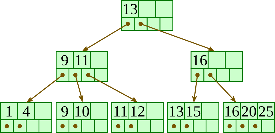
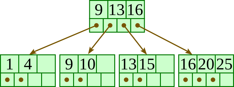
Here is a fairly small tree using 4 as our value for d.

A B+-tree requires that each leaf be the same distance from the root, as in this picture, where searching for any of the 11 values (all listed on the bottom level) will involve loading three nodes from the disk (the root block, a second-level block, and a leaf).

In practice, d will be larger — as large, in fact, as it takes to fill a disk block. Suppose a block is 4KB, our keys are 4-byte integers, and each reference is a 6-byte file offset. Then we'd choose d to be the largest value so that 4 (d − 1) + 6 d ≤ 4096; solving this inequality for d, we end up with d ≤ 410, so we'd use 410 for d. As you can see, d can be large.

A B+-tree maintains the following invariants:

Every node has one more references than it has keys.

All leaves are at the same distance from the root.

For every non-leaf node N with k being the number of keys in N: all keys in the first child's subtree are less than N's first key; and all keys in the ith child's subtree (2 ≤ i ≤ k) are between the (i − 1)th key of n and the ith key of n.

The root has at least two children.

Every non-leaf, non-root node has at least floor(d / 2) children.

Each leaf contains at least floor(d / 2) keys.

Every key from the table appears in a leaf, in left-to-right sorted order.

In our examples, we'll continue to use 4 for d. Looking at our invariants, this requires that each leaf have at least two keys, and each internal node to have at least two children (and thus at least one key).

10. Explain Insertion algorithm?

Descend to the leaf where the key fits.

If the node has an empty space, insert the key/reference pair into the node.

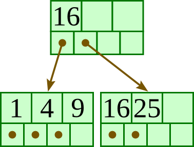
If the node is already full, split it into two nodes, distributing the keys evenly between the two nodes. If the node is a leaf, take a copy of the minimum value in the second of these two nodes and repeat this insertion algorithm to insert it into the parent node. If the node is a non-leaf, exclude the middle value during the split and repeat this insertion algorithm to insert this excluded value into the parent node.

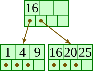
Initial:
Insert 20:
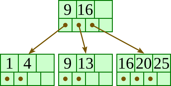
Insert 13:
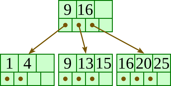
Insert 15:
Insert 10:
Insert 11:
Insert 12:

11. Explain the basic terminologies of graph?

Graph is a non-linear data structure. It contains a set of points known as nodes (or vertices) and a set of links known as edges (or Arcs). Here edges are used to connect the vertices. A graph is defined as follows...

Graph is a collection of vertices and arcs in which vertices are connected with arcs

Graph is a collection of nodes and edges in which nodes are connected with edges

Generally, a graph G is represented as G = ( V , E ), where V is set of vertices and E is set of edges.

Example

The following is a graph with 5 vertices and 6 edges.
This graph G can be defined as G = ( V , E )
Where V = {A,B,C,D,E} and E = {(A,B),(A,C)(A,D),(B,D),(C,D),(B,E),(E,D)}.

Graph Terminology

We use the following terms in graph data structure...

Vertex

Individual data element of a graph is called as Vertex. Vertex is also known as node. In above example graph, A, B, C, D & E are known as vertices.

Edge

An edge is a connecting link between two vertices. Edge is also known as Arc. An edge is represented as (startingVertex, endingVertex). For example, in above graph the link between vertices A and B is represented as (A,B). In above example graph, there are 7 edges (i.e., (A,B), (A,C), (A,D), (B,D), (B,E), (C,D), (D,E)).

Edges are three types.

Undirected Edge - An undirected egde is a bidirectional edge. If there is undirected edge between vertices A and B then edge (A , B) is equal to edge (B , A).

Directed Edge - A directed egde is a unidirectional edge. If there is directed edge between vertices A and B then edge (A , B) is not equal to edge (B , A).

Weighted Edge - A weighted egde is a edge with value (cost) on it.

Undirected Graph

A graph with only undirected edges is said to be undirected graph.

Directed Graph

A graph with only directed edges is said to be directed graph.

Mixed Graph

A graph with both undirected and directed edges is said to be mixed graph.

End vertices or Endpoints

The two vertices joined by edge are called end vertices (or endpoints) of that edge.

Origin

If a edge is directed, its first endpoint is said to be the origin of it.

Destination

If a edge is directed, its first endpoint is said to be the origin of it and the other endpoint is said to be the destination of that edge.

Adjacent

If there is an edge between vertices A and B then both A and B are said to be adjacent. In other words, vertices A and B are said to be adjacent if there is an edge between them.

Incident

Edge is said to be incident on a vertex if the vertex is one of the endpoints of that edge.

Outgoing Edge

A directed edge is said to be outgoing edge on its origin vertex.

Incoming Edge

A directed edge is said to be incoming edge on its destination vertex.

Degree

Total number of edges connected to a vertex is said to be degree of that vertex.

Indegree

Total number of incoming edges connected to a vertex is said to be indegree of that vertex.

Outdegree

Total number of outgoing edges connected to a vertex is said to be outdegree of that vertex.

Parallel edges or Multiple edges

If there are two undirected edges with same end vertices and two directed edges with same origin and destination, such edges are called parallel edges or multiple edges.

Self-loop

Edge (undirected or directed) is a self-loop if its two endpoints coincide with each other.

Simple Graph

A graph is said to be simple if there are no parallel and self-loop edges.

Path

A path is a sequence of alternate vertices and edges that starts at a vertex and ends at other vertex such that each edge is incident to its predecessor and successor vertex.

Sign Up