Unit - 3

Adversarial Search and Games

Q1) What is game theory?

A1) Game theory

Adversarial search is a sort of search that examines the problem that arises when we attempt to plan ahead of the world while other agents plan against us.

• In previous topics, we looked at search strategies that are purely associated with a single agent attempting to find a solution, which is often stated as a series of activities.
• However, in game play, there may be moments when more than one agent is looking for the same answer in the same search field.
• A multi-agent environment is one in which there are multiple agents, each of which is an opponent to the others and competes against them. Each agent must think about what another agent is doing and how that activity affects their own performance.
• Adversarial searches, also referred to as Games, are searches in which two or more players with conflicting goals try to find a solution in the same search space.
• The two fundamental variables that contribute in the modeling and solving of games in AI are a Search problem and a heuristic evaluation function.

Q2) What are the type of games in AI?

A2) Types of Games in AI

• Perfect information: A game with perfect information is one in which agents have complete visibility of the board. Agents can see each other's movements and have access to all game information. Examples include chess, checkers, go, and other games.
• Imperfect information: Tic-tac-toe, Battleship, blind, Bridge, and other games with incomplete information are known as such because the agents do not have all of the information and are unaware of what is going on.
• Deterministic games: Deterministic games have no element of chance and follow a strict pattern and set of rules. Examples include chess, checkers, go, tic-tac-toe, and other games.
• Non-deterministic games: Non-deterministic games are those with a number of unpredictable events and a chance or luck aspect. Dice or cards are used to introduce the element of chance or luck. These are unpredictably generated, and each action reaction is unique. Stochastic games are another name for these types of games.

Example: Backgammon, Monopoly, Poker, etc.

Q3) How to search for games?

A3) Searches in which two or more players with conflicting goals are trying to explore the same search space for the solution, are called adversarial searches, often known as Games.

Games are modeled as a Search problem and heuristic evaluation function, and these are the two main factors which help to model and solve games in AI.

Types of Games in AI:

• Perfect information: A game with the perfect information is that in which agents can look into the complete board. Agents have all the information about the game, and they can see each other moves also. Examples are Chess, Checkers, Go, etc.
• Imperfect information: If in a game agent do not have all information about the game and not aware with what's going on, such type of games are called the game with imperfect information, such as tic-tac-toe, Battleship, blind, Bridge, etc.
• Deterministic games: Deterministic games are those games which follow a strict pattern and set of rules for the games, and there is no randomness associated with them. Examples are chess, Checkers, Go, tic-tac-toe, etc.
• Non-deterministic games: Non-deterministic are those games which have various unpredictable events and has a factor of chance or luck. This factor of chance or luck is introduced by either dice or cards. These are random, and each action response is not fixed. Such games are also called as stochastic games.

Example: Backgammon, Monopoly, Poker, etc.

Zero-Sum Game

• Zero-sum games are adversarial search which involves pure competition.
• In Zero-sum game each agent's gain or loss of utility is exactly balanced by the losses or gains of utility of another agent.
• One player of the game try to maximize one single value, while other player tries to minimize it.
• Each move by one player in the game is called as ply.
• Chess and tic-tac-toe are examples of a Zero-sum game.

Zero-sum game: Embedded thinking

The Zero-sum game involved embedded thinking in which one agent or player is trying to figure out:

• What to do.
• How to decide the move
• Needs to think about his opponent as well
• The opponent also thinks what to do

Each of the players is trying to find out the response of his opponent to their actions. This requires embedded thinking or backward reasoning to solve the game problems in AI.

Formalization of the problem:

A game can be defined as a type of search in AI which can be formalized of the following elements:

• Initial state: It specifies how the game is set up at the start.
• Player(s): It specifies which player has moved in the state space.
• Action(s): It returns the set of legal moves in state space.
• Result(s, a): It is the transition model, which specifies the result of moves in the state space.
• Terminal-Test(s): Terminal test is true if the game is over, else it is false at any case. The state where the game ends is called terminal states.
• Utility(s, p): A utility function gives the final numeric value for a game that ends in terminal states s for player p. It is also called payoff function. For Chess, the outcomes are a win, loss, or draw and its payoff values are +1, 0, ½. And for tic-tac-toe, utility values are +1, -1, and 0.

Q4) What do you mean optimal decision in  games?

A4) Optimal decision in multiplayer games

A dependent strategy, which defines MAX's move in the initial state, then MAX's movements in the states resulting from every probable response by MIN (the opponent), and so on, is the optimal solution in adversarial search.

One move deep: If a game ends after one MAX and MIN move each, we say the tree is one move deep, with two half-moves, each referred to as a ply.

Minimax value: The node's minimax value is the utility (for MAX) of being in the corresponding state, assuming that both players play optimally from there until the game ends. The minimax value of a terminal state determines its utility.

Given a game tree, the optimal strategy can be computed using the minimax value of each node, i.e., MINIMAX (n).

MAX likes to get to the highest value state, whereas MIN prefers to go to the lowest value state.

Fig 1: Two ply game tree

Multiplayer games

Each node's single value must be replaced by a vector of values. A vector VA, VB, VC> is associated with each node in a three-player game with players A, B, and C, for example.

From each actor's perspective, this vector indicates the utility of a terminal circumstance.

In nonterminal states, the backed-up value of a node n is always the utility vector of the successor state with the highest value for the player choosing at n.

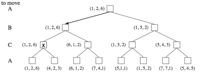
Fig 2: Three piles of a game tree with three players (A, B, C)

Q5) Explain heuristic alpha beta tree search?

A5) Alpha-beta pruning is a modified version of the minimax algorithm. It is an optimization technique for the minimax algorithm.

●      As we have seen in the minimax search algorithm that the number of game states it has to examine are exponential in depth of the tree. Since we cannot eliminate the exponent, but we can cut it to half. Hence there is a technique by which without checking each node of the game tree we can compute the correct minimax decision, and this technique is called pruning. This involves two threshold parameter Alpha and beta for future expansion, so it is called alpha-beta pruning. It is also called as Alpha-Beta Algorithm.

●      Alpha-beta pruning can be applied at any depth of a tree, and sometimes it not only prune the tree leaves but also entire sub-tree.

●      The two-parameter can be defined as:

1. Alpha: The best (highest-value) choice we have found so far at any point along the path of Maximizer. The initial value of alpha is -∞.
2. Beta: The best (lowest-value) choice we have found so far at any point along the path of Minimizer. The initial value of beta is +∞.

●      The Alpha-beta pruning to a standard minimax algorithm returns the same move as the standard algorithm does, but it removes all the nodes which are not really affecting the final decision but making algorithm slow. Hence by pruning these nodes, it makes the algorithm fast.

Condition for Alpha-beta pruning:

The main condition which required for alpha-beta pruning is:

α>=β 

Pseudo-code for Alpha-beta Pruning:

1. Function minimax(node, depth, alpha, beta, maximizingPlayer) is 
2. If depth ==0 or node is a terminal node then 
3. Return static evaluation of node 
4. If MaximizingPlayer then      // for Maximizer Player 
5. MaxEva= -infinity           
6. For each child of node do 
7. Eva= minimax(child, depth-1, alpha, beta, False) 
8. MaxEva= max(maxEva, eva)  
9. Alpha= max(alpha, maxEva)     
10. If beta<=alpha 
11. Break 
12. Return maxEva   
13. Else                         // for Minimizer player 
14. MinEva= +infinity  
15. For each child of node do 
16. Eva= minimax(child, depth-1, alpha, beta, true) 
17. MinEva= min(minEva, eva)  
18. Beta= min(beta, eva) 
19. If beta<=alpha 
20. Break         
21. Return minEva 

Q6) Explain the working of alpha beta pruning?

A6) Working of Alpha-Beta Pruning:

Let's take an example of two-player search tree to understand the working of Alpha-beta pruning

Step 1: At the first step the, Max player will start first move from node A where α= -∞ and β= +∞, these value of alpha and beta passed down to node B where again α= -∞ and β= +∞, and Node B passes the same value to its child D.

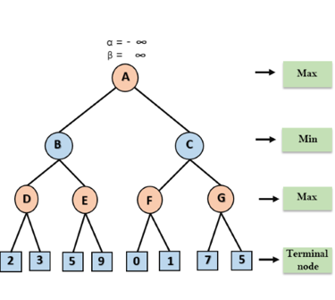
Step 2: At Node D, the value of α will be calculated as its turn for Max. The value of α is compared with firstly 2 and then 3, and the max (2, 3) = 3 will be the value of α at node D and node value will also 3.

Step 3: Now algorithm backtrack to node B, where the value of β will change as this is a turn of Min, Now β= +∞, will compare with the available subsequent nodes value, i.e. min (∞, 3) = 3, hence at node B now α= -∞, and β= 3.

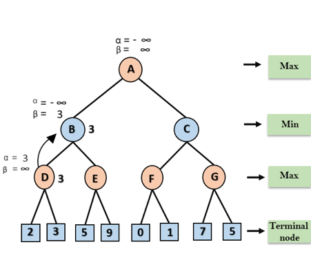
In the next step, algorithm traverse the next successor of Node B which is node E, and the values of α= -∞, and β= 3 will also be passed.

Step 4: At node E, Max will take its turn, and the value of alpha will change. The current value of alpha will be compared with 5, so max (-∞, 5) = 5, hence at node E α= 5 and β= 3, where α>=β, so the right successor of E will be pruned, and algorithm will not traverse it, and the value at node E will be 5.

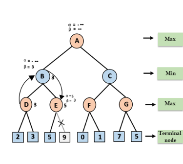
Step 5: At next step, algorithm again backtrack the tree, from node B to node A. At node A, the value of alpha will be changed the maximum available value is 3 as max (-∞, 3)= 3, and β= +∞, these two values now passes to right successor of A which is Node C.

At node C, α=3 and β= +∞, and the same values will be passed on to node F.

Step 6: At node F, again the value of α will be compared with left child which is 0, and max(3,0)= 3, and then compared with right child which is 1, and max(3,1)= 3 still α remains 3, but the node value of F will become 1.

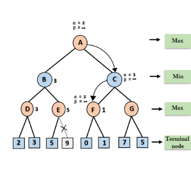
Step 7: Node F returns the node value 1 to node C, at C α= 3 and β= +∞, here the value of beta will be changed, it will compare with 1 so min (∞, 1) = 1. Now at C, α=3 and β= 1, and again it satisfies the condition α>=β, so the next child of C which is G will be pruned, and the algorithm will not compute the entire sub-tree G.

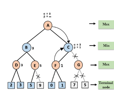
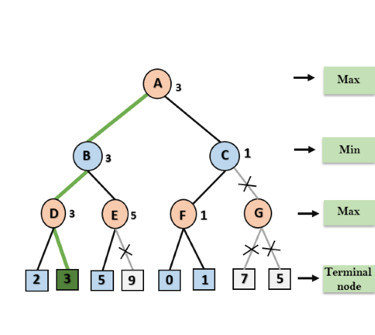
Step 8: C now returns the value of 1 to A here the best value for A is max (3, 1) = 3. Following is the final game tree which is the showing the nodes which are computed and nodes which has never computed. Hence the optimal value for the maximizer is 3 for this example.

Move Ordering in Alpha-Beta pruning:

The effectiveness of alpha-beta pruning is highly dependent on the order in which each node is examined. Move order is an important aspect of alpha-beta pruning.

It can be of two types:

●      Worst ordering: In some cases, alpha-beta pruning algorithm does not prune any of the leaves of the tree, and works exactly as minimax algorithm. In this case, it also consumes more time because of alpha-beta factors, such a move of pruning is called worst ordering. In this case, the best move occurs on the right side of the tree. The time complexity for such an order is O(bm).

●      Ideal ordering: The ideal ordering for alpha-beta pruning occurs when lots of pruning happens in the tree, and best moves occur at the left side of the tree. We apply DFS hence it first search left of the tree and go deep twice as minimax algorithm in the same amount of time. Complexity in ideal ordering is O(bm/2).

Rules to find good ordering:

Following are some rules to find good ordering in alpha-beta pruning:

●      Occur the best move from the shallowest node.

●      Order the nodes in the tree such that the best nodes are checked first.

●      Use domain knowledge while finding the best move. Ex: for Chess, try order: captures first, then threats, then forward moves, backward moves.

●      We can bookkeep the states, as there is a possibility that states may repeat.

Q7) Describe monte carlo search tree?

A7) Monte Carlo Tree Search (MCTS) is an artificial intelligence (AI) search strategy (AI). It's a probabilistic and heuristic-driven search method that blends traditional tree search implementations with reinforcement learning machine learning principles.

There's always the risk that the current best action isn't the most optimal action in tree search. In such instances, the MCTS algorithm comes in handy since it continues to assess other options occasionally during the learning phase by executing them instead of the currently perceived optimal approach. The "exploration-exploitation trade-off" is what it's called. It takes advantage of the actions and tactics that have been determined to be the most effective up to this point, but it must also continue to investigate the local space of alternative decisions to see if they may replace the present best.

Exploration aids in the exploration and discovery of the tree's unexplored areas, which may lead to the discovery of a more ideal path. To put it another way, inquiry broadens the tree's width rather than its depth. Exploration can help ensure that MCTS isn't missing out on any possibly better options. However, in cases involving a high number of steps or repeats, it quickly becomes inefficient. To avoid this, exploitation is used to balance things out.

Exploitation remains focused on a single path with the highest estimated value. This is a greedy technique, as it will increase the depth of the tree rather than its breadth. In basic terms, when applied to trees, the UCB formula helps to balance the exploration-exploitation trade-off by regularly examining relatively unknown nodes of the tree and discovering possibly more optimum paths than the one it is currently exploiting.

For this characteristic, MCTS becomes particularly useful in making optimal decisions in Artificial Intelligence (AI) problems.

Monte Carlo Tree Search (MCTS) algorithm:

The building blocks of the search tree in MCTS are nodes. These nodes are created using the results of several simulations. Monte Carlo Tree Search is divided into four steps: selection, expansion, simulation, and back propagation. Each of these steps is described in greater depth below:

Selection - The MCTS method uses a specific technique to explore the current tree from the root node. To choose the nodes with the highest estimated value, the technique employs an evaluation function. To traverse the tree, MCTS uses the Upper Confidence Bound (UCB) formula applied to trees as the approach in the selection process. It strikes a balance between exploration and exploitation. A node is chosen during tree traversal based on some parameters that return the highest value. The parameters are defined by the formula below, which is commonly used for this purpose.

Where;

Si = value of a node i

Xi = empirical mean of a node i

C = a constant

t = total number of simulations

The child node that returns the biggest value from the above equation will be selected when traversing a tree during the selection phase. When a child node that is also a leaf node is detected during traversal, the MCTS enters the expansion stage.

Expansion - A new child node is added to the tree to the node that was optimally attained during the selection process in this process.

Simulation - A simulation is carried out in this process by selecting moves or strategies until a desired result or condition is obtained.

Backpropagation - The remaining tree must be modified after finding the value of the newly inserted node. As a result, the backpropagation process is carried out, in which the new node propagates back to the root node. The amount of simulations kept in each node is increased during the procedure. The number of wins is also increased if the new node's simulation results in a win.

The actions outlined above can be visualised using the graphic below:

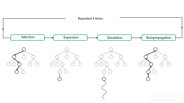
Fig 3: Outlined visualised graphics

These algorithms are especially beneficial in turn-based games like Tic Tac Toe, Connect 4, Checkers, Chess, Go, and others where there is no element of chance in the game rules. Artificial Intelligence Programs, such as AlphaGo, have lately employed this to compete against the world's best Go players. However, its use isn't confined to video games. It can be applied to any situation with state-action pairings and simulations to predict outcomes.

Q8) Define stochastic games?

A8) Stochastic games are simulations of dynamic interactions in which the environment changes in response to the activities of the participants. "In a stochastic game, the play progresses by steps from position to position, according to transition probabilities determined jointly by the two players," Shapley writes.

A group of participants participates in a stochastic game. At each stage of the game, the action takes place in a specific state (or position, in Shapley's terminology), and each player selects an action from a list of options. The stage payoff that each player receives is determined by the collection of actions that the players choose, as well as the current state, as well as a probability distribution for the subsequent state that the game will visit.

Stochastic games apply von Neumann's model of strategic-form games to dynamic settings in which the environment varies in response to the players' decisions. They also use the Markov decision problem model, which was created by numerous RAND Corporation researchers in 1949–1952, to competitive scenarios with multiple decision makers.

The complexity of stochastic games arises from the fact that the players' decisions have two, sometimes opposing, consequences. First, the players' actions, in combination with the present state, determine the immediate payment that each player receives. Second, the present state and the players' activities influence the next state selection, which influences future reward possibilities. Each player, in particular, must balance these factors when deciding on his actions, which might be a difficult decision.

Although this dichotomy is also present in one-player sequential decision problems, the presence of additional players who maximize their own goals adds complexity to the analysis of the situation.

Two player Games

For modelling and analysis of discrete systems functioning in an uncertain (adversarial) environment, stochastic two-player games on directed graphs are commonly employed. As vertices, a system's and its environment's possible configurations are represented, and transitions correspond to the system's, its environment's, or "nature's" actions. An infinite path in the graph corresponds to a run of the system. As a result, a system and its environment can be viewed as two hostile players, with one player (the system) aiming to maximise the probability of "good" runs and the other player (the environment) aiming to maximise the chance of "bad" runs.

Although there may be an equilibrium value for this probability in many circumstances, there may not be optimal solutions for both parties.

We go over some of the fundamental notions and algorithmic concerns that have been studied in this field, as well as some long-standing outstanding difficulties. Then we'll go through a few recent findings.

Application

Economic theory, evolutionary biology, and computer networks all use stochastic games. They are generalizations of repeated games that correspond to the unique case of a single state.

Q9) Write short notes on partially observable games?

A9) A partially observable stochastic game (POSG) is a tuple

{I, S, {b0}, {Ai}, {Oi},P, {Ri}i, where

●      I is a finite set of agents (or controllers) indexed 1, . . . , n.

●      S is a finite set of states.

●      b0 ∈ ∆(S) represents the initial state distribution

●      Ai is a finite set of actions available to agent i and A~ = ×i∈IAi is the set of joint actions (i.e., action profiles), where ~a = ha1, . . . , ani denotes a joint action

●      Oi is a finite set of observations for agent i and O~ = ×i∈IOi is the set of joint observations, where ~o = ho1, . . . , oni denotes a joint observation

●      P is a set of Markovian state transition and observation probabilities, where P(s 0 , ~o|s, ~a) denotes the probability that taking joint action ~a in state s results in a transition to state s 0 and joint observation ~o

●      Ri : S × A → < ~ is a reward function for agent i

A game unfolds across a finite or infinite number of stages, with the number of stages referred to as the game's horizon. We focus on finite-horizon POSGs in this study; some of the issues of solving the infinite-horizon situation are highlighted at the end. At each level, all agents choose an action at the same time and are rewarded and observed. Each agent's goal is to maximize the expected sum of prizes it will receive during the game. The reward functions determine whether agents compete or cooperate in their quest for a reward. A decentralized partially observable Markov decision process is one in which the agents share the same reward function.

Q10) Write the limitation of game search algorithms?

A10) Limitations of game search algorithms

●      The process of obtaining the goal is slower due to the large branching factor.

●      The engine's performance and efficiency suffer as a result of evaluating and searching all conceivable nodes and branches.

●      Both players have an excessive number of options from which to choose.

●      It is impossible to investigate the complete tree if there is a time and space constraint.

●      The biggest disadvantage of the minimax algorithm is that it becomes extremely slow while playing complex games like chess or go. This style of game contains a lot of branching, and the player has a lot of options to choose from.

The algorithm, however, can be enhanced by Alpha-Beta Pruning.

Q11) What is CSP?

A11) A constraint satisfaction problem (CSP) consists of

●        A set of variables,

●        A domain for each variable, and

●        A set of constraints.

The aim is to choose a value for each variable so that the resulting possible world satisfies the constraints; we want a model of the constraints.

A finite CSP has a finite set of variables and a finite domain for each variable. Many of the methods considered in this chapter only work for finite CSPs, although some are designed for infinite, even continuous, domains.

The multidimensional aspect of these problems, where each variable can be seen as a separate dimension, makes them difficult to solve but also provides structure that can be exploited.

Given a CSP, there are a number of tasks that can be performed:

●        Determine whether or not there is a model.

●        Find a model.

●        Find all of the models or enumerate the models.

●        Count the number of models.

●        Find the best model, given a measure of how good models are.

●        Determine whether some statement holds in all models.

This mostly considers the problem of finding a model. Some of the methods can also determine if there is no solution. What may be more surprising is that some of the methods can find a model if one exists, but they cannot tell us that there is no model if none exists.

CSPs are very common, so it is worth trying to find relatively efficient ways to solve them. Determining whether there is a model for a CSP with finite domains is NP-hard and no known algorithms exist to solve such problems that do not use exponential time in the worst case. However, just because a problem is NP-hard does not mean that all instances are difficult to solve. Many instances have structure that can be exploited.

Q12) Describe constraints propagation?

A12) The constraints are used in a number of inference approaches to determine which variable/value combinations are consistent and which are not. Node, arc, path, and k-consistent are examples of these.

Constraint propagation: Using constraints to reduce the number of permissible values for one variable, which then reduces the number of legal values for another variable, and so on.

Local consistency: If we treat each variable as a node in a graph and each binary constraint as an arc, the act of enforcing local consistency in each area of the graph eliminates inconsistent values across the board.

Different types of local consistency exist:

Node consistency

●      If all of the values in the variable's domain fulfil the variable's unary constraint, the variable is node-consistent (a node in the CSP network).

●      If every variable in a network is node-consistent, we call it a node-consistent network.

Arc consistency

●      If every value in a variable's domain fulfils the variable's binary constraints, the variable is arc-consistent in a CSP.

●      If there is some value in the domain Dj that satisfies the binary constraint on the arc for every value in the current domain Di, then Xi is arc-consistent with regard to another variable Xj (Xi, Xj).

●      If every variable in a network is arc-consistent with every other variable, it is said to be arc-consistent.

●      Using the arcs, arc consistency tightens the domains (unary constraint) (binary constraints).

AC-3 algorithm

Function AC-3(csp) returns false if an inconsistency is found and true otherwise

Inputs: csp, a binary  CSP with components (X, D, C)

Local variables: queue, a queue of arcs, initially all the arcs in csp

While queue is not empty do

If REVISE(csp, ) then

If  size of then return false

For each in NEIGHBORS - do

Add to queue

Return true

Function REVISE (csp, returns true iff we revise the domain of

Revised false

For each x in do

If no value in allows (x,y) to satisfy the constraint between and then

Delete from

Revised true

Return revised

This is arc consistency algorithm

●      AC-3 keeps an arc queue that initially contains all of the arcs in the CSP.

●      Then, from the queue, AC-3 selects an arbitrary arc (Xi, Xj) and makes Xi arc-consistent with respect to Xj.

●      If Di remains unchanged, continue on to the next arc; if Di is revised, add any arcs (Xk, Xi) where Xk is a neighbour of Xi to the queue.

●      If Di is reduced to zero, the entire CSP will collapse since there is no consistent answer.

●      Otherwise, keep checking and removing values from variable domains until there are no more arcs in the queue.

●      As a result, an arc-consistent CSP with smaller domains has the same solutions as the original.

The complexity of AC-3:

Assume a CSP with n variables, each with domain size at most d, and with c binary constraints (arcs). Checking consistency of an arc can be done in O(d2) time, total worst-case time is O(cd3)

Path consistency

●      A two-variable set Xi, Xj is path-consistent with regard to a third variable Xm if there is an assignment to Xm that fulfils the constraints on Xi, Xm, and Xm, Xj for every assignment Xi = a, Xj = b consistent with the constraint on Xi, Xj.

●      The binary restrictions are tightened by path consistency, which uses implicit constraints inferred from triples of variables.

K-consistency

●      A CSP is k-consistent if a consistent value can always be assigned to any kth variable for any collection of k-1 variables and for any consistent assignment to those variables.

●      1-consistency = node consistency; 2-consistency = arc consistency; 3-consistency = path consistency.

●      If a CSP is k-consistent and also (k – 1)-consistent, (k – 2)-consistent,... All the way down to 1-consistent, it is very k-consistent.

●      We can ensure that if we take a CSP with n nodes and make it strongly n-consistent, we will discover a solution in time O(n2d). However, in the worst situation, the procedure for establishing n-consistency must take time exponential in n and demand space exponential in n.

Global constraints

A global constraint is one that applies to an infinite number of variables (but not necessarily all variables). Special-purpose algorithms that are more efficient than general-purpose approaches can manage global constraints.

1) inconsistency detection for Alldiff constraints

A straightforward formula is as follows: Remove any variable with a singleton domain from the constraint and delete its value from the domains of the remaining variables. Repeat for as long as singleton variables exist. An inconsistency has been discovered if an empty domain is formed at any stage or if there are more variables than domain values left.

Applying arc consistency to an analogous collection of binary constraints is sometimes more effective than using a simple consistency approach for a higher-order constraint.

2) inconsistency detection for resource constraint (the atmost constraint)

●      By calculating the total of the current domains' minimum values, we may find inconsistencies.

●      e.g., Atmost(10, P1, P2, P3, P4): a total of no more than 10 workers is assigned.

●      The Atmost constraint cannot be met if each variable has the domain 3, 4, 5, 6.

●      We can ensure consistency by eliminating any domain's maximum value if it differs from the minimum values of the other domains.

●      For example, if the domains of each variable in the example are 2, 3, 4, 5, 6, the values 5 and 6 can be removed from each domain.

3) inconsistency detection for bounds consistent

Domains are represented by upper and lower limits and handled via bounds propagation for big resource-limited issues with integer values.

e.g - In an airline-scheduling problem, imagine there are two flights F1 and F2, each with a capacity of 165 and 385 passengers. The initial domains for passenger numbers on each aircraft are

D1 = [0, 165] and D2 = [0, 385].

Assume we also have the limitation that the two flights must each carry 420 passengers: F1 + F2 = 420. We reduce the domains to, by propagating bounds constraints.

D1 = [35, 165] and D2 = [255, 385].

If there is a value of Y that fulfills the constraint between X and Y for every variable Y, and for both the lower-bound and upper-bound values of X, a CSP is bound  consistent.

Q13) Define backtracking search for CSP?

A13) CSPs are frequently solved via backtracking search, a type of depth-first search. Inference and search can be combined.

Commutativity: All CSPs are commutative. A issue is commutative if the sequence in which a series of activities is carried out has no bearing on the outcome.

Backtracking search: A depth-first search that assigns values to one variable at a time and then backtracks when there are no more legal values to assign to that variable.

The backtracking algorithm selects an unassigned variable each time and then attempts all of the values in that variable's domain in order to discover a solution. If an inconsistency is found, BACKTRACK fails, leading the previous call to try a different value.

There is no need to provide a domain-specific initial state, action function, transition model, or goal test to BACKTRACKING-SEARCH.

BACKTRACKING-SEARCH maintains only one representation of a state and modifies it rather than producing new ones.

Function BACTRACKING-SEARCH(csp) returns a solution, or failure

Return BACTRACK({}, csp)

VarSELECT-UNASSIGNED-VARIABLE(csp)

For each value in ORDER-DOMAIN-VALUES(var,assignement,csp) do

If value is consistent with assignment then

Add{var=value} to assignment

Inferences INFERENCE(csp,var,value)

If inferences failure then

Add inferences to assignment

Result BACKTRACK (assignment, csp)

If result failure then

Return result

Remove {var=value} and inferences from assignment

Return failure

This is simple backtracking algorithm for CSP

Address the following questions to efficiently answer CSPs without domain-specific knowledge:

Which variable should be assigned next, according to the SELECT-UNASSIGNED-VARIABLE function?

What order should the values of the ORDER-DOMAIN-VALUES function be tested in?

2)INFERENCE FUNCTION: What inferences should be made at each stage of the search?

3)Can the search avoid repeating its failure when it comes across an assignment that violates a constraint?

1. Variable and value ordering

SELECT-UNASSIGNED-VARIABLE

Variable selection—fail-first

Minimum-remaining-values (MRV) heuristic: The concept of selecting the variable having the smallest number of "legal" values. The "most constrained variable" or "fail-first" heuristic selects a variable that is most likely to cause a failure soon, allowing the search tree to be pruned. If a variable X has no more permissible values, the MRV heuristic will select X, and failure will be noticed instantly, avoiding the need for fruitless searches through other variables.

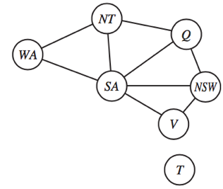
For example, since there is only one potential value for SA after WA=red and NT=green, it makes logical to assign SA=blue next rather than Q.

Degree heuristic: By selecting the variable that is implicated in the greatest number of constraints on other unassigned variables, the degree heuristic seeks to lower the branching factor on future decisions.

SA, for example, has the highest degree of 5; the other variables have degrees of 2 or 3; and T has a degree of 0.

ORDER-DOMAIN-VALUES

Value selection—fail-last

If we're looking for all possible solutions to a problem (rather than simply the first one), the order doesn't matter.

Least-constraining-value heuristic: chooses the value that eliminates the fewest options for the constraint graph's surrounding variables. (Leave as much freedom as possible for subsequent variable assignments.)

For example, we've created a partial assignment with WA=red and NT=green, and Q is our next option. Because blue eliminates the final lawful value available for Q's neighbour, SA, who prefers red to blue, it is a negative decision.

In a backtracking search, the minimum-remaining-values and degree heuristics are domain-independent approaches for determining which variable to choose next. The least-constraining-value heuristic aids in determining which value for a given variable to try first.

2. Interleaving search and inference

INFERENCE

Forward chaining - [One of the simplest forms of inference is forward checking.] When a variable X is assigned, the forward-checking method creates arc consistency for it: delete from Y's domain any value that is inconsistent with the value chosen for X for each unassigned variable Y that is associated to X by a constraint.

If we've previously done arc consistency as a preprocessing step, there's no reason to do forward checking.

Fig 4: Progress of a map coloring search with forward checking

Advantage: Combining the MRV heuristic with forward checking will make the search more effective for many issues.

Disadvantages: Forward checking only makes the current variable arc-consistent, not all the other variables.

MAC (Maintaining Arc Consistency) algorithm: [Detect this inconsistency more effectively than forward checking.] The INFERENCE function invokes AC-3 once a variable Xi is allocated a value, but instead of a queue of all arcs in the CSP, we only start with the arcs(Xj, Xi) for those Xj that are unassigned variables that are neighbours of Xi. The call to AC-3 then proceeds as usual, with the exception that if any variable's domain is reduced to the empty set, the call to AC-3 fails and we know to retrace immediately.

3. Intelligent backtracking

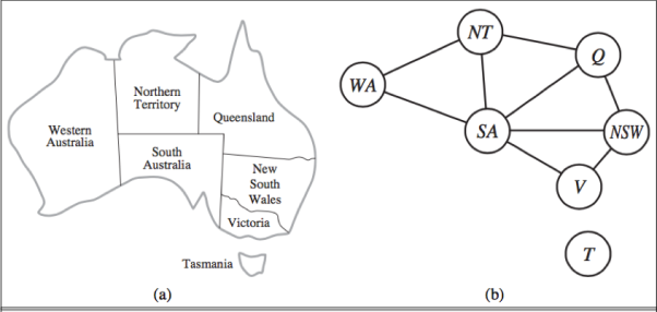
Fig 5: (a) Principal states and territories of Australia. Colouring this map can be viewed as CSP. (b) the map coloring problem represented as a constraint graph

Chronological backtracking: Figure shows the BACKGRACING-SEARCH. If a branch of the search fails, go back to the previous variable and try a different value for it. (The most recent point of decision is revisited.)

For example, consider the partial assignment Q=red, NSW=green, V=blue, T=red.

When we attempt the next variable, SA, we notice that every value breaks a constraint.

We go back to T and try a different hue, but it doesn't work.

Intelligent backtracking: Return to the variable that caused one of the possible values of the following variable (e.g. SA) to be impossible.

A collection of assignments for a variable that are in conflict with some value for that variable.

(For example, the conflict set for SA is Q=red, NSW=green, V=blue.)

Backtracks to the most recent assignment in the conflict set using the backjumping approach.

(e.g - Backjumping, for example, would leap over T and try a different value for V.)

Forward checking can supply the conflict set with no extra work.

Add X=x to Y's conflict set whenever forward checking based on an assignment X=x deletes a value from Y's domain.

If the last value in Y's domain is removed, the assignments in Y's conflict set are added to X's conflict set.

In reality, forward checking prunes every branch cut by backjumping. In a forward-checking search or a search that uses stronger consistency checking, basic backjumping is thus superfluous (such as MAC).

Q14) Where is the game theory now?

A14) Game Theory is increasingly becoming a part of the real-world in its various applications in areas like public health services, public safety, and wildlife. Currently, game theory is being used in adversary training in GANs, multi-agent systems, and imitation and reinforcement learning. In the case of perfect information and symmetric games, many Machine Learning and Deep Learning techniques are applicable. The real challenge lies in the development of techniques to handle incomplete information games, such as Poker. The complexity of the game lies in the fact that there are too many combinations of cards and the uncertainty of the cards being held by the various players.