Unit - 5
Expectation Maximization
Q1) What do you mean BY Expectation Maximization?
A1) Expectation Maximization
In the real-world applications of machine learning, it is very common that there are many relevant features available for learning but only a small subset of them are observable. So, for the variables which are sometimes observable and sometimes not, then we can use the instances when that variable is visible is observed for learning and then predict its value in the instances when it is not observable.
On the other hand, the Expectation-Maximization algorithm can be used for the latent variables (variables that are not directly observable and are inferred from the values of the other observed variables) too to predict their values with the condition that the general form of probability distribution governing those latent variables is known to us. This algorithm is actually at the base of many unsupervised clustering algorithms in the field of machine learning.
It was explained, proposed, and given its name in a paper published in 1977 by Arthur Dempster, Nan Laird, and Donald Rubin. It is used to find the local maximum likelihood parameters of a statistical model in the cases where latent variables are involved and the data is missing or incomplete.
Algorithm:
Given a set of incomplete data, consider a set of starting parameters.
Expectation step (E – step): Using the observed available data of the dataset, estimate (guess) the values of the missing data.
Maximization step (M – step): Complete data generated after the expectation (E) step is used to update the parameters.
Repeat step 2 and step 3 until convergence
The essence of the Expectation-Maximization algorithm is to use the available observed data of the dataset to estimate the missing data and then using that data to
Update the values of the parameters. Let us understand the EM algorithm in detail.
Initially, a set of initial values of the parameters are considered. A set of incomplete observed data is given to the system with the assumption that the observed data comes from a specific model.
The next step is known as “Expectation” – step or E-step. In this step, we use the observed data to estimate or guess the values of the missing or incomplete data. It is used to update the variables.
The next step is known as “Maximization”-step or M-step. In this step, we use the complete data generated in the preceding “Expectation” – step to update the values of the parameters. It is used to update the hypothesis.
Now, in the fourth step, it is checked whether the values are converging or not, if yes, then stop otherwise repeat step-2 and step-3 i.e. “Expectation” – step and “Maximization” – step until the convergence occurs.
Q2) Write advantages and disadvantages of EM?
A2) Advantages of EM algorithm
● It is always guaranteed that likelihood will increase with each iteration.
● The E-step and M-step are often pretty easy for many problems in terms of
Implementation.
● Solutions to the M-steps often exist in the closed-form.
Disadvantages of EM algorithm
● It has slow convergence.
● It makes convergence to the local optima only.
● It requires both the probabilities, forward and backward (numerical
● optimization requires only forward probability).
Q3) Explain GMMs?
A3) GMMs
Suppose there are K clusters (For the sake of simplicity here it is assumed that the number of clusters is known and it is K) (For the sake of simplicity here it is assumed that the number of clusters is known and it is K). So μand Σ are also calculated for each k. Had it been just one distribution, they would have been calculated by the maximum-likelihood method. But since there are K such clusters and the probability density is defined as a linear function of densities of all these K distributions, i.e.


For estimating the parameters by maximum log-likelihood method, compute
p(X|μ, Σ, 兀)


Now define a random variable 𝞬k(X) such that 𝞬k(X) = p(k|X).
From Bayes’ theorem,


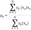
Now for the log probability function to be optimum, its derivative of p(X|μ, Σ, 兀) with respect to μ, Σ and 兀 should be zero. So equaling the derivative of p(X|μ, Σ, 兀) with respect to μ to zero and rearranging the terms,

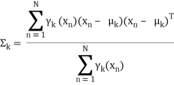
Similarly taking derivatives with respect to Σ and 兀respectively, one can obtain the following expressions.


 denotes the total number of sampling points in the k-th cluster. Here it is assumed that there is a total N number of samples and each sample containing d features is denoted by xi .
So it can be clearly seen that the parameters cannot be calculated in closed form. This is where Expectation - Maximization algorithm is useful.
Q4) What is the usage of the EM algorithm?
A4) Usage of EM Algorithm
● It can be used to fill the missing data in a sample.
● It can be used as the basis of unsupervised learning of clusters.
● It can be used to estimate the parameters of the Hidden Markov Model (HMM).
● It can be used for discovering the values of latent variables.
Q5) What do you mean by Bayesian Networks?
A5) Bayesian Network
An alternative is to build a model that maintains known conditional dependency between random variables and conditional independence in all other cases. Bayesian networks are a probabilistic graphical model that specifically capture the known conditional dependency with directed edges in a graph model. All missing connections describe the conditional independencies in the model.
As such Bayesian Networks provide a useful tool to visualise the probabilistic model for a domain, review all of the relationships between the random variables, and reason about causal probabilities for scenarios given available proof.
Bayesian networks are a type of probabilistic graphical model comprised of nodes and directed edges.
Bayesian network models capture both conditionally dependent and conditionally independent relationships between random variables.
Models can be prepared by experts or learned from data, then used for inference to estimate the probabilities for causal or subsequent events.
Designing a Bayesian Network requires defining at least three things:
● Random Variables. What are the random variables in the problem?
● Conditional Relationships. What are the conditional relationships between the variables?
● Probability Distributions. What are the probability distributions for each variable?
It may be possible for an expert in the problem domain to specify some or all of these aspects in the design of the model.
In many cases, the architecture or topology of the graphical model can be specified by an expert, but the probability distributions must be estimated from data from the domain.
Both the probability distributions and the graph structure itself can be estimated from data, although it can be a challenging process. As such, it is common to use learning algorithms for this purpose; for example, assuming a Gaussian distribution for continuous random variables gradient ascent for estimating the distribution parameters.
When a Bayesian Network has been prepared for a domain, it can be used for reasoning, e.g. Making decisions.
Reasoning is accomplished by inference with the model for a given situation. For example, the outcome for certain events is known and plugged into the random variables. The model can be used to predict the likelihood of triggers for the events or potential further outcomes.
Q6) Write any example of a Bayesian network?
A6) Example of Bayesian Network
We can render Bayesian Networks concrete with a small example.
Consider a dilemma with three random variables: A, B, and C. A is dependent upon B, and C is dependent upon B.
We may state the conditional dependencies as follows:
● A is conditionally dependent upon B, e.g. P(A|B)
● C is conditionally dependent upon B, e.g. P(C|B)
We know that C and A have no impact on each other.
We may also state the conditional independencies as follows:
● A is conditionally independent from C: P(A|B, C)
● C is conditionally independent from A: P(C|B, A)
Note that the conditional dependency is specified in the presence of the conditional independence. That is, A is conditionally independent of C, or A is conditionally dependent upon B in the presence of C.
We can also state the conditional independence of A given C as the conditional dependence of A given B, as A is unaffected by C and can be determined from A given B alone.
P(A|C, B) = P(A|B)
We can see that B is unaffected by A and C and has no parents; we can clearly state the conditional freedom of B from A and C as P(B, P(A|B), P(C|B)) or P(B) (B).
We can also write the joint probability of A and C given B or conditioned on B as the product of two conditional probabilities;
For example:
P(A, C | B) = P(A|B) * P(C|B)
The model summarises the joint probability of P(A, B, C), calculated as:
P(A, B, C) = P(A|B) * P(C|B) * P(B)
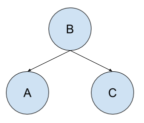
We can draw the graph as follows:

Fig 1: simple bayesian network
Q7) Describe reinforcements learning?
A7) Reinforcements Learning
Reinforcement learning (RL) solves a particular kind of problem were decision making is sequential, and the goal is long-term, such as game playing, robotics, resource management, or logistics.
RL is an area of Machine Learning which is related to taking suitable action to maximize reward in a particular situation. It is employed by various software and machines to find the best possible behaviour or path. RL differs from supervised learning in a way that the training data has the answer key with it so the model is trained with the correct answer itself whereas in reinforcement learning, there is no answer but the reinforcement agent decides what to do to perform the given task. In the absence of a training dataset, it is bound to learn from its experience.
Example:
For a robot, an environment is a place where it has been put to use. Remember this, the robot is itself the agent. For example, a textile factory where a robot is used to move materials from one place to another.
These tasks have a property in common: these tasks involve an environment and expect the agents to learn from that environment. This is where traditional machine learning fails and hence the need for reinforcement learning.
q-learning
Q-learning is another type of reinforcement learning algorithm that seeks to find the best action to take given the current state. It’s considered as the off-policy because the q-learning function learns from actions that are outside the current policy, such as taking random actions, and therefore a policy isn’t needed.
More specifically, q-learning seeks to learn a policy that maximizes the total reward.
Role of ‘Q’
The ‘q’ in q-learning stands for quality. Quality in this case represents how useful a given action is in gaining some future reward.
Create a q-table
When q-learning is performed we create what’s called a q-table or matrix that follows the shape of [state, action] and we initialize our values to zero. We then update and store our q-values after an episode. This q-table becomes a reference table for our agent to select the best action based on the q-value.
Updating the q-table
The updates occur after each step or action and end when an episode is done. Done in this case means reaching some terminal point by the agent. A terminal state for example can be anything like landing on a checkout page, reaching the end of some game, completing some desired objective, etc. The agent will not learn much after a single episode, but eventually, with enough exploring (steps and episodes) it will converge and learn the optimal q-values or q-star (Q∗).
Here are the 3 basic steps:
- The agent starts in a state (s1) takes an action (a1) and receives a reward (r1)
- The agent selects action by referencing Q-table with the highest value (max) OR by random (epsilon, ε)
- Update q-values