Unit - 1
Random Processes & Noise
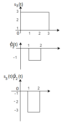
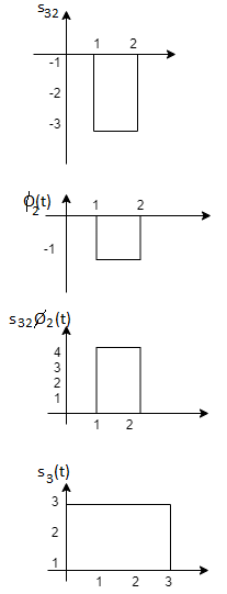
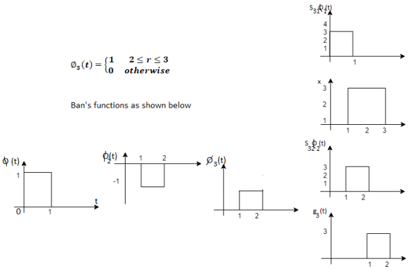
Q1) Using the fram-schmidt orthogonalization procedure, find a set of orthonormal ban’s functions represent the tree signals  as shown in figure.
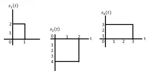
A1)
All the three signals  are not linear combination of each other hence they are linearly independent. Hence, we require three ban’s function.
To obtain 
Energy of 


To obtain 


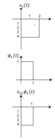


To obtain 





Q2) Consider the signals  and
and as given below. Find an orthonormal basis for phase set of signals using Grammar schimdt orthogonalisation procedure.
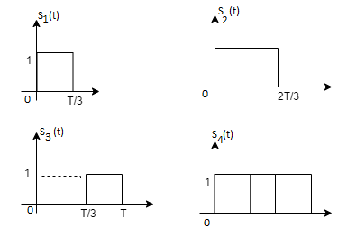
Fig. Sketch of  and
and 
A2)
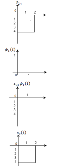
From the above figures  . This means all four signals are not linearly independent. Gram-schmidt orthogonalisation procedure is carried out for a subset which is linearly independent. Here
  are linearly independent. Hence, we will determine orthonormal.
To obtain 
Energy of  is
is 


We know that


To obtain 


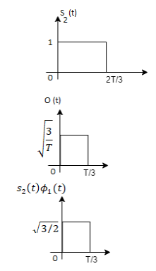

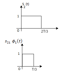
From the above figure the intermediate function can be defined as

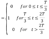
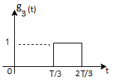
Energy of  will be


Now


To obtain 
We know that the generalized equation for gramm-scmidt procedure

With N=3


We know that


Since, there is no overlap between  and
and 

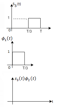


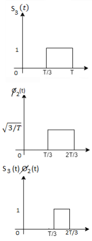
Here 


We know that


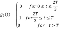

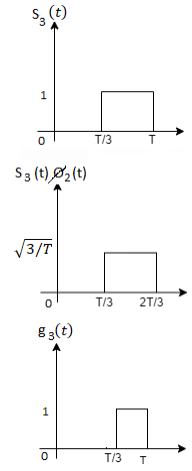


Figure below shows orthonormal basis function

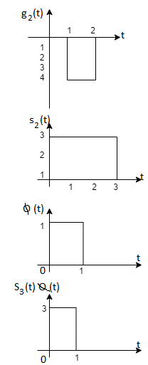
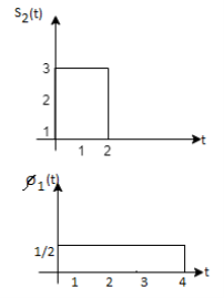
Q3) Three signals  are shown in fig. Apply Gram-schmidt procedure to obtain an orthonormal basis for the signals. Express signals
  in terms of orthonormal basis function.

A3)
i) To obtain orthonormal basis function
Here 
Hence, we will obtain basis solution for  and
and  only.
only.
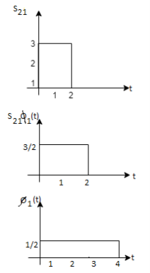
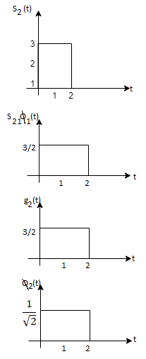
To obtain 
Energy of  is
is 


We know that

To obtain 






Q4) What are random signals?
A4) Random signals and noise are present in several engineering systems. Practical signals seldom lend themselves to a nice mathematical deterministic description. It is partly a consequence of the chaos that is produced by nature. However, chaos can also be man-made, and one can even state that chaos is a condition sine qua non to be able to transfer information. Signals that are not random in time but predictable contain no information, as was concluded by Shannon in his famous communication theory.
A (one-dimensional) random process is a (scalar) function y(t), where t is usually time, for which the future evolution is not determined uniquely by any set of initial data or at least by any set that is knowable to you and me. In other words, random process" is just a fancy phrase that means unpredictable function". Random processes y takes on a continuum of values ranging over some interval, often but not always - to +. The generalization to y's with discrete (e.g., integral) values is straightforward
Examples of random processes are:
(i) The total energy E(t) in a cell of gas that is in contact with a heat bath;
(ii) The temperature T(t) at the corner of Main Street and Center Street in Logan, Utah;
(iii) The earth-longitude (t) of a specific oxygen molecule in the earth's atmosphere.
One can also deal with random processes that are vector or tensor functions of time. Ensembles of random processes. Since the precise time evolution of a random process is not predictable, if one wishes to make predictions one can do so only probabilistically. The foundation for probabilistic predictions is an ensemble of random processes |i.e., a collection of a huge number of random processes each of which behaves in its own, unpredictable way. The probability density function describes the general distribution of the magnitude of the random process, but it gives no information on the time or frequency content of the process. Ensemble averaging and Time averaging can be used to obtain the process properties.
Q5) Explain correlation and covariance function?
A5) Correlation
The covariance has units (units of X times units of Y), and thus it can be difficult to assess how strongly related two quantities are. The correlation coefficient is a dimensionless quantity that helps to assess this.
The correlation coefficient between X and Y normalizes the covariance such that the resulting statistic lies between -1 and 1. The Pearson correlation coefficient is

The correlation matrix for X and Y is

Covariance
If we have two samples of the same size, X_i, and Y_i, where i=1,…,n, then the covariance is an estimate of how variation in X is related to variation in Y. The covariance is defined as

Where mu_X is the mean of the X sample, and mu_Y is the mean of the Y sample. Negative covariance means that smaller X tend to be associated with larger Y (and vice versa). Positive covariance means that larger/smaller X are associated with larger/smaller Y. Note that the covariance of X and Y is exactly the same as the covariance of Y and X. Also note that the covariance of X with itself is the variance of X. The covariance matrix for X and Y is thus

Q6) What is meant by ergodic process?
A6)
• In econometrics and signal processing, a stochastic process is said to be ergodic if its statistical properties can be deduced from a single, sufficiently long, random sample of the process.
• The reasoning is that any collection of random samples from a process must represent the average statistical properties of the entire process.
• In other words, regardless of what the individual samples are, a birds-eye view of the collection of samples must represent the whole process.
• Conversely, a process that is not ergodic is a process that changes erratically at an inconsistent rate.
Q7) Let X(t)be a zero-mean WSS process with RX(τ)=e−|τ|. X(t)is input to an LTI system with
|H(f)|=√ (1+4π2f2) |f|<2
= 0 otherwise,
Let Y(t) be the output.
- Find μY(t)=E[Y(t)]
- Find RY(τ)
- Find E[Y(t)2]
A7) Note that since X(t)is WSS, X(t)and Y(t)are jointly WSS, and therefore Y(t)is WSS.
- To find μY(t), we can write
μY=μXH(0) =0*1= 0
b. To find RY(τ), we first find SY(f)
SY(f)=SX(f)|H(f)|2
From Fourier transform tables, we can see that
SX(f)=F{e−|τ|} =2/(1+(2πf)2)
Then, we can find SY(f)as
SY(f)=SX(f)|H(f)|2
=2|f|<2
= 0 otherwise
We can now find RY(τ)by taking the inverse Fourier transform of SY(f)
RY(τ)=8sinc(4τ),
Where
Sinc(f)=sin(πf)/πf
c. We have
E[Y(t)2] = RY (0) =8.
Q8) What is internal noise and its types?
A8) The term noise is used customarily to designate unwanted signals that tend to disturb the transmission and processing of signals in communication systems, and over which we have incomplete control. In practice, we find that there are many potential sources of noise in a communication system. The sources of noise may be external to the system (e.g., atmospheric noise, galactic noise, man-made noise) or internal to the system. The second category includes an important type of noise that arises from the phenomenon of spontaneous fluctuations of current flow that is experienced in all electrical circuits. In a physical context, the most common examples of the spontaneous fluctuation phenomenon are shot noise which arises because of the discrete nature of current flow in electronic devices; and thermal noise, which is attributed to the random motion of electrons in a conductor.
Internal Noise
Also called fundamental noise which is originated within electronic devices or circuits. They are called fundamental sources because they are the integral part of the physical nature of the material used for making electronic components.
This type of noise follows certain rules. Therefore, it can be eliminated by properly designing the electronic circuits and equipment.
The fundamental noise sources produce different types of noise. They are as follows.
(i) Thermal noise
(ii) Shot noise
(iii) Partition noise
(iv) Low frequency or flicker noise
(v) High frequency or transit time noise
Q9) A noise generator using diode is required to produce 15µV noise voltage in a receiver which has an input impedance of 75Ω (Purely resistive). The receiver has a noise power bandwidth of 200KHz calculate the current through the diode.
A9) Given Vn = 15µV
R = 75Ω
B = 200 KHz
Noise current flowing through 75Ω is

= 0.2X10-6
= 0.2µa
Diode current –short noise current is given by
I2n = 2 (I +Io) qB
I2n= 2I X Q X B (neglecting Io)
(0.2 X 10⁻⁶) 2 = 2I X 1.6 X 10-19 X 200 X 103
I = 0.625 A = 625 µA
Q10) A receiver has a noise power band width of 12KHz. A register which watch with the receiver input impedance is connected across the antenna terminals what is the noise power contributed by this register in the receiver bandwidth. Assume temperature to be 30ºC
A10) Given: B = kHz; T = 30ºC = 30+ 273 = 303 K
Pn = KTB
= 1.38 X 10-23 X 303 X 12 X 103
= 5.01768 X 10⁻¹⁷ W
Q11) Write short notes on flicker noise and high frequency noise?
A11) The flicker noise appears at frequencies below a few kHz it is sometimes called as 1/f noise in the semiconductor devices, the flicker noise is generated due to the fluctuations in the carrier density.
These fluctuations in the carrier density will cause the fluctuation in the conductivity of the material. This will produce a fluctuating voltage drop when a direct-current flow through a device this fluctuating voltage is called as flicker noise voltage.
The mean square value of flicker noise voltage is proportional to the square of direct current flowing through the device.
High frequency noise Also called Transit time noise
If the time taken by an electron to travel from the emitter to the collector of a transistor becomes comparable to the period of the signal which is being period of the signal which is being amplified then the transit time effect takes place.
This effect is observed at every high frequency. Due to the transit time effect some of the carriers may diffuse back to the emitter. This gives rise to an input admittance, the conductance component of which increases with frequency.
The minute current induced in the input of the device by the random fluctuations in the output current, will create random noise at high frequencies
Q12) Explain Johnson noise?
A12) Thermal Noise Also known as Johnson Noise.
The free electrons with in a conductor are always in random motion.
This random motion is due to the thermal energy received by them. The distribution of these free electrons with in a conductor at a given instant of time is not uniform.
It is possible that an excess number of electrons may appears at one end or the other of the conductor
The average voltage resulting from this non uniform distribution is zero but the average power is not zero
As this power results from the thermal energy are called as the “Thermal noise power”
The average thermal noise power is given by
Pn = KTB Watts
Where: k = Boltzmann’s constant = 1.38 X 10⁻²³ J/K
B = Bandwidth of the noise spectrum (Hz)
T = Temperature of the conductor in K
The thermal noise power Pn in proportional to the noise BW and conductor temperature
Q13) What is noise? Also explain shot noise?
A13) The term noise is used customarily to designate unwanted signals that tend to disturb the transmission and processing of signals in communication systems, and over which we have incomplete control. In practice, we find that there are many potential sources of noise in a communication system. The sources of noise may be external to the system (e.g., atmospheric noise, galactic noise, man-made noise) or internal to the system. The second category includes an important type of noise that arises from the phenomenon of spontaneous fluctuations of current flow that is experienced in all electrical circuits. In a physical context, the most common examples of the spontaneous fluctuation phenomenon are shot noise which arises because of the discrete nature of current flow in electronic devices; and thermal noise, which is attributed to the random motion of electrons in a conductor.
Internal Noise
Also called fundamental noise which is originated within electronic devices or circuits. They are called fundamental sources because they are the integral part of the physical nature of the material used for making electronic components.
This type of noise follows certain rules. Therefore, it can be eliminated by properly designing the electronic circuits and equipment.
The fundamental noise sources produce different types of noise. They are as follows.
(i) Thermal noise
(ii) Shot noise
(iii) Partition noise
(iv) Low frequency or flicker noise
(v) High frequency or transit time noise
Shot Noise
It is produced due to shot effect. Due to the shot effect shot noise is produced in all the amplifying devices rather in all the active devices.
The shot noise is produced due to the random variations in the arrival of electronics (or holes) at the output electrode of an amplifying devices.
Therefore, it appears as a randomly varying noise current superimposed and the output. The shot noise “Sounds” like a shower of lead shots falling on a metal sheet.
The shot noise has a uniform spectral density like thermal noise
The mean square shot noise current for a diode is given as
In2 = 2 (J + Io) qB Amp2
Where I = direct current across the junction in amperes
Io = reverse saturation current in ampere
q = electron charge = 1.6 X 10⁻¹⁹ C
B = Effective noise Band width in Hz
Q14) Explain superposition of noise?
A14) The equations derived in above section represents the noise as a superposition of noise spectral components. The frequency of these components is  f and
f and  f tends to 0. The nth noise component can be given as


The spectral components of noise are random processes. The variables an, bn, Dn and ɸn are random variables. As nn(t) is random process the normalised power of nn(t) can be found by taking average of [nn(t)]2.

Substituting value of nn(t) and finding normalised power we get

As nn(t) is stationary process value of 
At time t=t1 cos (2πn ft1) =1 and sin (2πn
 ft1) =0.

At time t=t2 cos (2πn ft1) =0 and sin (2πn
 ft1) =1.


 ]
]

But


The average of multiplication of two terms in above equation is nothing but correlation between them.
Consider two noise components n1(t) and n2(t). Then the total noise due to these components is
n(t) = n1(t)+ n2(t)
This is called superposition.
The normalised power P of these components is given as


The term  represents the cross correlation of n1(t) and n2(t). As individual spectral components of Gaussian noise are uncorrelated hence the correlation of n1(t) and n2(t) will be zero.


Q15) Explain linear filtering of noise?
A15) Noise has wide range of frequencies. Generally, we use filters to minimize the noise power. These filters are narrow filters and they pass the frequencies of the required signals. The noise power is reduced in the output of the filter. These filters are used before the demodulators in the receivers. The filters used in noise for linear filtering are:
RC-Low Pass Filter
The transfer function of RC filter is given

fc = 3db cut-off frequency of the filters.
Considering ni(t) with PSD of Si(f) and output noise signal be no(t) with PSD of So(f). The output and input PSDs of noise

If the input noise is additive white gaussian noise (AWGN), the PSDs we have,

The magnitude of H(f) can be obtained from

Substituting the values, we get

The equation gives power spectral density of output noise signal. The average power can be obtained from PSD

The expression for output noise power is given as


Let x=f/fc


The average noise power at the output of RC filter is

Ideal Low Pass Filter
The transfer function of ideal LPF is given as


The input and output PSD are given as


The value of average noise power at output is given as


The above equation is the noise power at the output of ideal LPF.
Q16) What is quadrature component of noise?
A16) The spectral component of noise is represented as

Another way of representing the noise is shown below

The above equation of noise is also called as narrowband representation of noise because there is narrow frequency band at the neighbour of frequency fo. The quadrature component representation is also used because of the appearance in the equation of sinusoids in quadrature. Let fo corresponds to k=k’ we get
fo =k
The term 2πfot- 2π k t =0 is added to above equation we get

Using some trigonometric identities for cosine and sine terms we can also write above equation as


The variables nc(t) and ns(t) are stationary random processes represented as linear superposition of spectral components. The narrow band noise can be seen in relation to find out the quadrature component of noise. The noise spectral component in n(t) of frequency f= k gives rise in nc(t) and ns(t) to a spectral component of frequency (k-K)
  = f-fo
If we assume the noise n(t) is narrow band and extends over bandwidth B and also is selected midway in the frequency range of the noise. The noise spectrum of n(t) extends from fo-B/2 to fo+B/2. The spectrum of nc(t) and ns(t) extends over -B/2 to +B/2. In view of the slow variation of nc(t) and ns(t) relative to the sinusoid of frequency fo it is useful to give the quadrature representation of noise as interpretation in terms of phasors and a phasor diagram. The term nc(t)cos2πfot is of frequency fo and has varying amplitude of nc(t). The term -ns(t)sin2πfot is in quadrature with first term and has slow varying amplitude ns(t). In coordinate system rotating counter-clockwise with angular velocity 2πfo with phasor diagram shown below.
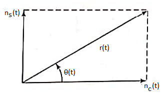
Fig: A phasor diagram of Quadrature representation of noise
The two phasors of varying amplitude give rise to third resultant phasor of amplitude r(t) = [nc2(t)+ns2(t)]1/2
And having angle shown below.

Q17) Why frequency domain representation of noise is generally preferred?
A17)
The frequency domain representation of signal makes the analysis simple. The system performance is affected due to presence of these unwanted signals in form of noise. So, to make our study easy we use frequency domain analysis for study of noise. Consider a sample noise signal shown below having interval of T. A periodic noise is generated after T interval. The Fourier Series representation of the signal is given as
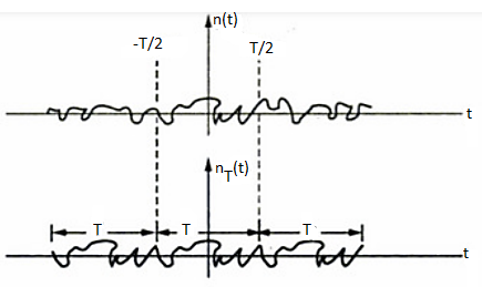
Fig: Sample noise waveform

 i.e., signal of Fig.3.6.1(b)
 assuming that noise signal has no d.c. Component
 i.e., period of noise signal
The above equation can be written as


The polar form of Fourier series is represented as


 and
and 


By Parseval’s Theorem


The average power P is area under the power spectral density curve


For one component


The above equation gives the PSD at frequency component n f where
  f = 1/T

By Fourier Series relation we have


The above equations give the PSD for frequency components n f. The power spectrum is shown below.
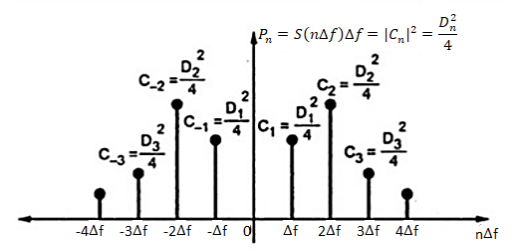
Fig: Power Spectrum
The above derivation was made by assuming noise as a periodic signal. But the fact is noise is never periodic. Now, considering T tends to infinity and  f tends to 0. The actual noise will then be


The above equation represents noise in frequency domain. The values of constants an and bn are changing as noise is not constant. Hence, they are called random variables of noise, then we write  in place of an and
  in place of an.

As  f tends to 0 the discrete spectral lines and power spectrum gets closer and forms continuous spectrum.


Q18) Explain LTI system with random inputs?
A18) LTI Systems with Random Inputs:
Consider an LTI system with impulse response h(t). Let X(t) be a WSS random process. If X(t) is the input of the system, then the output, Y(t), is also a random process. More specifically, we can write
Y(t)=h(t)∗X(t)=
Here, our goal is to show that X(t) and Y(t) are jointly WSS processes. Let's first start by calculating the mean function of Y(t), μY(t). We have
μY(t)=E[Y(t)]
=E [ ]
]
=
=
=μX
We note that μY(t)is not a function of t, so we can write
μY(t)=μY=μX .
.
Let's next find the cross-correlation function, RXY(t1, t2).
We have
RXY(t1, t2) =E[X(t1)Y(t2)]=E[X(t1) ]
]
=E[
=
=
= (since X(t) is WSS).
We note that RXY(t1, t2)is only a function of τ=t1−t2, so we may write
RXY(τ)=
=h(τ)∗RX(−τ)
=h(−τ) ∗ RX(τ).
Similarly, you can show that
RY(τ)=h(τ)∗h(−τ) ∗ RX(τ).
From the above results we conclude that X(t)and Y(t)are jointly WSS.