Unit - 6

Introduction to 1D & 2D Signal Processing

Q1)

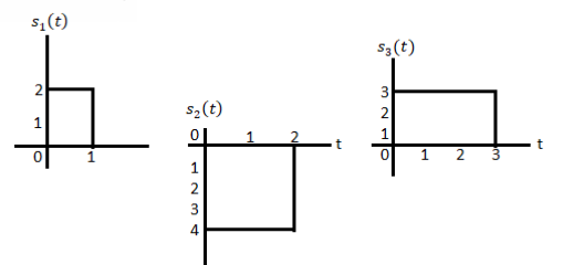
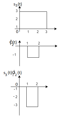
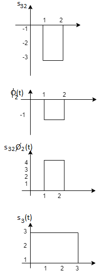
Using the fram-schmidt orthogonalization procedure, find a set of orthonormal ban’s functions represent the tree signals as shown in figure.

A1)

All the three signals are not linear combination of each other hence they are linearly independent. Hence we require three ban’s function.

To obtain

Energy of

To obtain

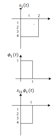
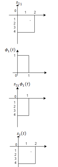
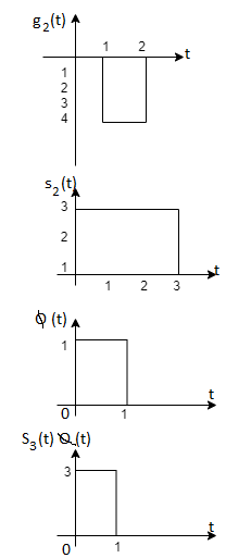
To obtain

Q2)

Consider the signals andas given below. Find an orthonormal basis for phase set of signals using Grammar schimdt orthogonalisation procedure.

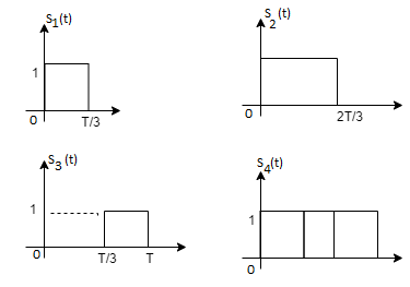
Fig. Sketch of and

A2)

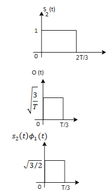
From he above figures . This means all four signals are not linearly independent. Gram-schmidt orthogonalisation procedure is carried out for a subset which is linearly independent. Here are linearly independent. Hence we will determine orthonormal.

To obtain

Energy of is

We know that

To obtain

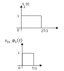
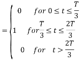
From the above figure the intermediate function can be defined as

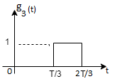
Energy of will be

Now

To obtain

We know that the generalized equation for gramm-scmidt procedure

With N=3

We know that

Since, there is no overlap between and

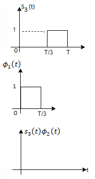
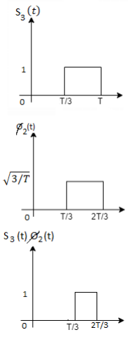
Here

We know that

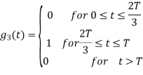
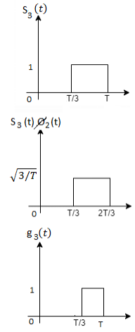
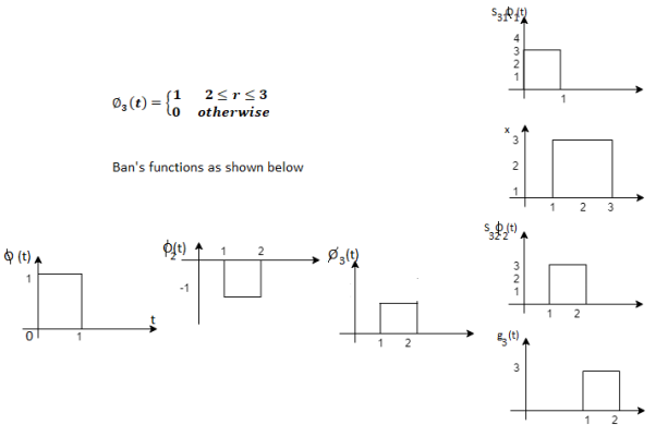
Figure below shows orthonormal basis function

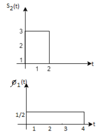
Q3) Three signals are shown in fig. Apply Gram-schmidt procedure to obtain an orthonormal basis for the signals. Express signals in terms of orthonormal basis function.

A3)

i) To obtain orthonormal basis function

Here

Hence we will obtain basis solution for and only.

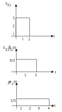
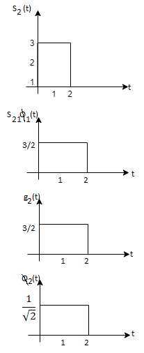
To obtain

Energy of is

We know that

To obtain

Q4) Explain the human vocal tract mechanism with proper figure?

A4)

Vocal tract —dotted lines in figure; begins at the glottis (the vocal cords) and ends at the lips. Consists of the pharynx (the connection from the oesophagus to the mouth) and the mouth itself (the oral cavity). Average male vocal tract length is 17.5 cm. Cross sectional area, determined by positions of the tongue, lips, jaw and velum, varies from zero (complete closure) to 20 sq cm Nasal tract — begins at the velum and ends at the nostrils Velum —a trapdoor-like mechanism at the back of the mouth cavity; lowers to couple the nasal tract to the vocal tract to produce the nasal sounds like /m/ (mom), /n/ (night), /ng/ (sing).

1.When the vocal cords are tensed, the air flow causes them to vibrate, producing voiced sound.

2. When the vocal cords are relaxed, in order to produce a sound, the air flow either must pass through a constriction in the vocal tract and there by become turbulent, producing unvoiced sound or it can build up pressure behind a point of total closure within the vocal tract and when the closure is opened, the pressure is suddenly and abruptly released, causing a brief transient sound.

The shape of the vocal tract transforms raw sound from the vocal folds into recognizable sounds.

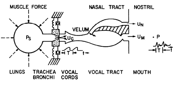
Fig: Abstraction of Physical Model

A schematic longitudinal cross-sectional drawing of the human vocal tract mechanism is given in Figure above. This diagram highlights the essential physical features of human anatomy that enter into the final stages of the speech production process. It shows the vocal tract as a tube of nonuniform cross-sectional area that is bounded at one end by the vocal cords and at the other by the mouth opening. This tube serves as an acoustic transmission system for sounds generated inside the vocal tract.

For creating nasal sounds like /M/, /N/, or /NG/, a side-branch tube, called the nasal tract, is connected to the main acoustic branch by the trapdoor action of the velum. This branch path radiates sound at the nostrils. The shape (variation of cross-section along the axis) of the vocal tract varies with time due to motions of the lips, jaw, tongue, and velum. Although the actual human vocal tract is not laid out along a straight line as in Figure above, this type of model is a reasonable approximation for wavelengths of the sounds in speech.

Q5) What are voiced and unvoiced sounds explain them?

A5) The sounds of speech are generated in the system of Figure above in several ways. Voiced sounds (vowels, liquids, glides, nasals) are produced when the vocal tract tube is excited by pulses of air pressure resulting from quasi-periodic opening and closing of the glottal orifice (opening between the vocal cords). Examples are the vowels /UH/, /IY/, and /EY/, and the liquid consonant /W/.

Unvoiced sounds are produced by creating a constriction somewhere in the vocal tract tube and forcing air through that constriction, thereby creating turbulent air flow, which acts as a random noise excitation of the vocal tract tube. Examples are the unvoiced fricative sounds such as /SH/ and /S/. A third sound production mechanism is when the vocal tract is partially closed off causing turbulent flow due to the constriction, at the same time allowing quasi-periodic flow due to vocal cord vibrations. Sounds produced in this manner include the voiced fricatives /V/, /DH/, /Z/, and /ZH/. Finally, plosive sounds such as /P/, /T/, and /K/ and affricates such as /CH/ are formed by momentarily closing off air flow, allowing pressure to build up behind the closure, and then abruptly releasing the pressure. All these excitation sources create a wide-band excitation signal to the vocal tract tube, which acts as an acoustic transmission line with certain vocal tract shape-dependent resonances that tend to emphasize some frequencies of the excitation relative to others.

Q6) How are speech signals represented. Draw block diagram and explain each of them?

A6)

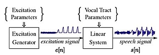
Fig: Speech Signal Representation

The discrete-time time-varying linear system on the right in Figure above simulates the frequency shaping of the vocal tract tube. The excitation generator on the left simulates the different modes of sound generation in the vocal tract. Samples of a speech signal are assumed to be the output of the time-varying linear system.

In general such a model is called a source/system model of speech production. The short-time frequency response of the linear system simulates the frequency shaping of the vocal tract system, and since the vocal tract changes shape relatively slowly, it is reasonable to assume that the linear system response does not vary over time intervals on the order of 10 ms or so. Thus, it is common to characterize the discrete-time linear system by a system function of the form:

Where the filter coefficients ak and bk (labeled as vocal tract parameters in Figure above) change at a rate on the order of 50–100 times/s. Some of the poles (ck) of the system function lie close to the unit circle and create resonances to model the formant frequencies. In detailed modeling of speech production, it is sometimes useful to employ zeros (dk) of the system function to model nasal and fricative sounds.

The box labelled excitation generator in Figure above creates an appropriate excitation for the type of sound being produced. For voiced speech the excitation to the linear system is a quasi-periodic sequence of discrete (glottal) pulses that look very much like those shown in the righthand half of the excitation signal waveform in Figure above. The fundamental frequency of the glottal excitation determines the perceived pitch of the voice. The individual finite-duration glottal pulses have a lowpass spectrum that depends on a number of factors. Therefore, the periodic sequence of smooth glottal pulses has a harmonic line spectrum with components that decrease in amplitude with increasing frequency. Often it is convenient to absorb the glottal pulse spectrum contribution into the vocal tract system model.

This can be achieved by a small increase in the order of the denominator over what would be needed to represent the formant resonances. For unvoiced speech, the linear system is excited by a random number generator that produces a discrete-time noise signal with flat spectrum as shown in the left-hand half of the excitation signal. The excitation in Figure above switches from unvoiced to voiced leading to the speech signal output as shown in the figure. In either case, the linear system imposes its frequency response on the spectrum to create the speech sounds.

This model of speech as the output of a slowly time-varying digital filter with an excitation that captures the nature of the voiced/unvoiced distinction in speech production is the basis for thinking about the speech signal, and a wide variety of digital representations of the speech signal are based on it. That is, the speech signal is represented by the parameters of the model instead of the sampled waveform. By assuming that the properties of the speech signal (and the model) are constant over short time intervals, it is possible to compute/measure/estimate the parameters of the model by analysing short blocks of samples of the speech signal. It is through such models and analysis techniques that we are able to build properties of the speech production process into digital representations of the speech signal.

Q7) How we can calculate the fundamental frequency of speech signal. Give the proper formula?

A7) The fundamental frequency of a speech signal, often denoted by F0 or F0, refers to the approximate frequency of the (quasi-)periodic structure of voiced speech signals. The oscillation originates from the vocal folds, which oscillate in the airflow when appropriately tensed. The fundamental frequency is defined as the average number of oscillations per second and expressed in Hertz. Typically, fundamental frequencies lie roughly in the range 80 to 450 Hz, where males have lower voices than females and children. The F0 of an individual speaker depends primarily on the length of the vocal folds, which is in turn correlated with overall body size.

If F0 is the fundamental frequency, then the length of a single period in seconds is

T=1/f0

The speech waveform thus repeats itself after every T seconds.

A simple way of modelling the fundamental frequency is to repeat the signal after a delay of T seconds. If a signal is sampled with a sampling rate of Fs, then the signal repeats after a delay of L samples where:

L=Fs T= Fs/F0

Q8) What are random signals?

A8) Random signals and noise are present in several engineering systems. Practical signals seldom lend themselves to a nice mathematical deterministic description. It is partly a consequence of the chaos that is produced by nature. However, chaos can also be man-made, and one can even state that chaos is a condition sine qua non to be able to transfer information. Signals that are not random in time but predictable contain no information, as was concluded by Shannon in his famous communication theory.

A (one-dimensional) random process is a (scalar) function y(t), where t is usually time, for which the future evolution is not determined uniquely by any set of initial data or at least by any set that is knowable to you and me. In other words, random process" is just a fancy phrase that means unpredictable function". Random processes y takes on a continuum of values ranging over some interval, often but not always - to +. The generalization to y's with discrete (e.g., integral) values is straightforward

Examples of random processes are:

(i) the total energy E(t) in a cell of gas that is in contact with a heat bath;

(ii) the temperature T(t) at the corner of Main Street and Center Street in Logan, Utah;

(iii) the earth-longitude (t) of a specific oxygen molecule in the earth's atmosphere.

One can also deal with random processes that are vector or tensor functions of time. Ensembles of random processes. Since the precise time evolution of a random process is not predictable, if one wishes to make predictions one can do so only probabilistically. The foundation for probabilistic predictions is an ensemble of random processes |i.e., a collection of a huge number of random processes each of which behaves in its own, unpredictable way. The probability density function describes the general distribution of the magnitude of the random process, but it gives no information on the time or frequency content of the process. Ensemble averaging and Time averaging can be used to obtain the process properties.

Q9) Explain noise cancellation using adaptive filters?

A9) Adaptive Noise Canceller (ANC) removes or suppresses noise from a signal using adaptive filters that automatically adjust their parameters. The ANC uses a reference input derived from single or multiple sensors located at points in the noise field where the signal is weak or undetectable. Adaptive filters then determine the input signal and decrease the noise level in the system output. The parameters of the adaptive filter can be adjusted automatically and require almost neither prior signal information nor noise characteristics. However, the computational requirements of adaptive filters are very high due to long impulse responses, especially during implementation on digital signal processors. Convergence becomes very slow if the adaptive filter receives a signal with high spectral dynamic range such as in non-stationary environments and colored background noise. In the last few decades, numerous approaches have been proposed to overcome these issues.

For example, the Wiener filter, Recursive-Least-Square (RLS) algorithm, and the Kalman filter were proposed to achieve the best performance of adaptive filters. Apart from these algorithms, the Least Mean Square (LMS) algorithm is most commonly used because of its robustness and simplicity. However, the LMS suffers from significant performance degradation with colored interference signals. Other algorithms, such as the Affine Projection algorithm (APA), became alternative approaches to track changes in background noise; but its computational complexity increases with the projection order, limiting its use in acoustical environments.

An adaptive filtering system derived from the LMS algorithm, called Adaptive Line Enhancer (ALE), was proposed as a solution to the problems stated above. ALE is an adaptive self-tuning filter capable of, separating the periodic and stochastic components in a signal. The ALE detects extremely low-level sine waves in noise, and may be applied in speech with noisy environment. Furthermore, unlike ANCs, ALEs do not require direct access to the noise nor a way of isolating noise from the useful signal. In literature, several ALE methods have been proposed for acoustics applications. These methods mainly focus on improving the convergence rate of the adaptive algorithms using modified filter designs, realized as transversal Finite Impulse Response (FIR), recursive Infinite Impulse Response (IIR), lattice, and sub-band filters.

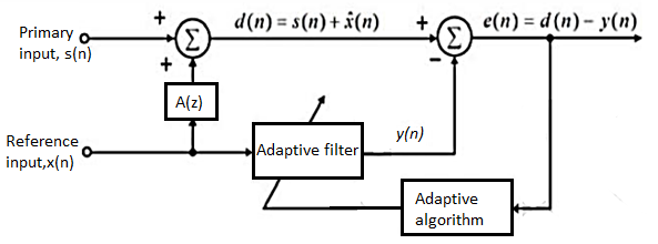
Fig: Block diagram of adaptive noise cancellation system

It is shown that for this application of adaptive noise cancellation, large filter lengths are required to account for a highly reverberant recording environment and that there is a direct relation between filter mis-adjustment and induced echo in the output speech. The second reference noise signal is adaptively filtered using the least mean squares, LMS, and the lattice gradient algorithms. These two approaches are compared in terms of degree of noise power reduction, algorithm convergence time, and degree of speech enhancement.

The effectiveness of noise suppression depends directly on the ability of the filter to estimate the transfer function relating the primary and reference noise channels. A study of the filter length required to achieve a desired noise reduction level in a hard-walled room is presented. Results demonstrating noise reduction in excess 10dB in an environment with 0dB signal noise ratio.

Q10) What is smoothing. What is the need for smoothing signal? Explain the soothing algorithm also?

A10) In many experiments in physical science, the true signal amplitudes (y-axis values) change rather smoothly as a function of the x-axis values, whereas many kinds of noise are seen as rapid, random changes in amplitude from point to point within the signal. In the latter situation it may be useful in some cases to attempt to reduce the noise by a process called smoothing. In smoothing, the data points of a signal are modified so that individual points that are higher than the immediately adjacent points (presumably because of noise) are reduced, and points that are lower than the adjacent points are increased. This naturally leads to a smoother signal. As long as the true underlying signal is actually smooth, then the true signal will not be much distorted by smoothing, but the noise will be reduced.

Most smoothing algorithms are based on the "shift and multiply" technique, in which a group of adjacent points in the original data are multiplied point-by-point by a set of numbers (coefficients) that defines the smooth shape, the products are added up to become one point of smoothed data, then the set of coefficients is shifted one point down the original data and the process is repeated. The simplest smoothing algorithm is the rectangular or unweighted sliding-average smooth; it simply replaces each point in the signal with the average of m adjacent points, where m is a positive integer called the smooth width. For example, for a 3-point smooth (m=3).

For j = 2 to n-1, where Sj the jth point in the smoothed signal, Yj the jth point in the original signal, and n is the total number of points in the signal. Similar smooth operations can be constructed for any desired smooth width, m.

Usually, m is an odd number. If the noise in the data is "white noise" (that is, evenly distributed over all frequencies) and its standard deviation is s, then the standard deviation of the noise remaining in the signal after the first pass of an unweighted sliding-average smooth will be approximately s over the square root of m (s/sqrt(m)), where m is the smooth width. The triangular smooth is like the rectangular smooth, above, except that it implements a weighted smoothing function. For a 5-point smooth (m = 5)

For j = 3 to n-2, and similarly for other smooth widths. It is often useful to apply a smoothing operation more than once, that is, to smooth an already smoothed signal, in order to build longer and more complicated smooths. For example, the 5-point triangular smooth above is equivalent to two passes of a 3-point rectangular smooth. Three passes of a 3-point rectangular smooth result in a 7-point "pseudo-Gaussian" or haystack smooth.

Q11) What is ECG? Explain the basics of ECG?

A11) The electrocardiogram (ECG) is used to monitor the proper functioning of heart. The electric signals from the muscle fibres are changed due to stimulation of muscle alters. Cardiac cells, unlike other cells, have a property known as automaticity, which is the capacity to spontaneously initiate impulses. These are then transmitted from cell to cell by gap junctions that connect cardiac cells to each other. The electrical impulses spread through the muscle cells because of changes in ions between intracellular and extracellular fluid. This is referred to as action potential. The primary ions involved are potassium, sodium and calcium. The action potential is the potential for action created by the balance between electrical charges (positive and negative) of ions on either side of the cell membrane. When the cells are in a resting state, the insides are negatively charged compared to the outsides.

Membrane pumps act to maintain this electrical polarity (negative charge) of the cardiac cells. Contraction of the heart muscle is triggered by depolarisation, which causes the internal negative charge to be lost transiently. These waves of depolarisation and repolarisation represent an electrical current and can be detected by placing electrodes on the surface of the body. After the current has spread from the heart through the body, the changes are picked up by the ECG machine and the activity is recorded on previously sensitised paper. The ECG is therefore a graphic representation of the electrical activity in the heart. The current is transmitted across the ECG machine at the selected points of contact of the electrode with the body.

Q12) What are artifacts? Also mention the techniques use to suppress them?

A12) Artifacts (noise) are the unwanted signals that are merged with ECG signal and sometimes create obstacles for the physicians from making a true diagnosis. Hence, it is necessary to remove them from ECG signals using proper signal processing methods. There are mainly four types of artifacts encountered in ECG signals: baseline wander, powerline interference, EMG noise and electrode motion artifacts.

Baseline Wander

Baseline wander or baseline drift is the effect where the base axis (x-axis) of a signal appears to ‘wander’ or move up and down rather than be straight. This causes the entire signal to shift from its normal base. In ECG signal, the baseline wander is caused due to improper electrodes (electrode-skin impedance), patient’s movement and breathing (respiration). Figure shows a typical ECG signal affected by baseline wander. The frequency content of the baseline wander is in the range of 0.5 Hz. However, increased movement of the body during exercise or stress test increase the frequency content of baseline wander. Since the baseline signal is a low frequency signal therefore Finite Impulse Response (FIR) high-pass zero phase forward-backward filtering with a cut-off frequency of 0.5 Hz to estimate and remove the baseline in the ECG signal can be used.

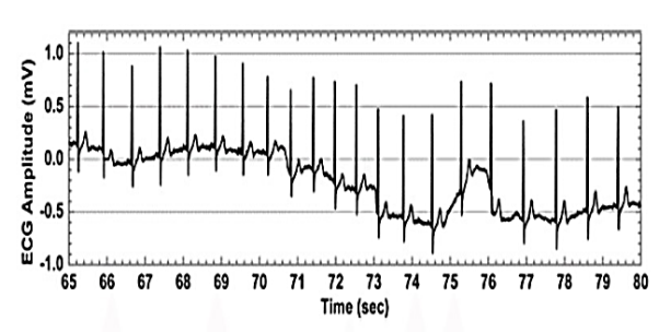
Fig: ECG Signal with baseline wander

Powerline Interference

Electromagnetic fields caused by a powerline represent a common noise source in the ECG, as well as to any other bioelectrical signal recorded from the body surface. Such noise is characterized by 50 or 60 Hz sinusoidal interference, possibly accompanied by a number of harmonics. Such narrowband noise renders the analysis and interpretation of the ECG more difficult, since the delineation of low-amplitude waveforms becomes unreliable and spurious waveforms may be introduced. It is necessary to remove powerline interference from ECG signals as it completely superimposes the low frequency ECG waves like P wave and T wave.

Q13) What are EMG noise and electrode motion artifacts?

A13) EMG Noise

The presence of muscle noise represents a major problem in many ECG applications, especially in recordings acquired during exercise, since low amplitude waveforms may become completely obscured. Muscle noise is, in contrast to baseline wander and 50/60 Hz interference, not removed by narrowband filtering, but presents a much more difficult filtering problem since the spectral content of muscle activity considerably overlaps that of the PQRST complex. Since the ECG is a repetitive signal, techniques can be used to reduce muscle noise in a way similar to the processing of evoked potentials. Successful noise reduction by ensemble averaging is, however, restricted to one particular QRS morphology at a time and requires that several beats be available. Hence, there is still a need to develop signal processing techniques which can reduce the influence of muscle noise [4]. Figure below shows an ECG signal interfered by an EMG noise.

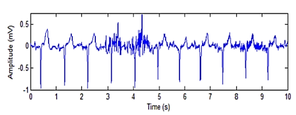
Fig: ECG signal with electromyographic (EMG) noise

Electrode Motion Artifacts

Electrode motion artifacts are mainly caused by skin stretching which alters the impedance of the skin around the electrode. Motion artifacts resemble the signal characteristics of baseline wander, but are more problematic to combat since their spectral content considerably overlaps that of the PQRST complex. They occur mainly in the range from 1 to 10 Hz. In the ECG, these artifacts are manifested as large-amplitude waveforms which are sometimes mistaken for QRS complexes. Electrode motion artifacts are particularly troublesome in the context of ambulatory ECG monitoring where they constitute the main source of falsely detected heartbeats.

Q14) How artifacts are removed using baseline wander method and power line interference?

A14) Techniques for Removal of Baseline Wander

A straightforward approach to the design of a filter is to choose the ideal high-pass filter as a starting Point.

Point. 

Since the corresponding impulse response has an infinite length, truncation can be done by multiplying h(n) by a rectangular window function, defined by or by another window function if more appropriate. Such an FIR filter should have an order 2L + 1.

Wavelet transform can also be used to remove the baseline wander from ECG signal. The frequency of baseline wander is approximately 0.5 Hz. According to discrete wavelet transform (DWT), the original signal is to be decomposed using the subsequent low-pass filters (LPF) and high-pass filters (HPF). The cut-off frequency for LPF and HPF will be half of the sampling frequency.

Techniques for Removal of Powerline Interference

A very simple approach to the reduction of powerline interference is to consider a filter defined by a complex conjugated pair of zeros that lie on the unit circle at the interfering frequency.

Such a second-order FIR filter has the transfer function

Since this filter has a notch with a relatively large bandwidth, it will attenuate not only the powerline frequency but also the ECG waveforms with frequencies close to ω0. It is, therefore, necessary to modify the filter so that the notch becomes more selective, for example, by introducing a pair of complex conjugated poles positioned at the same angle as the zeros, but at a radius r

Where 0 <1< r . Thus, the transfer function of the resulting IIR filter is given by

The notch bandwidth is determined by the pole radius r and is reduced as r approaches the unit circle. The impulse response and the magnitude function for two different values of the radius, r = 0.75 and 0.95. From Figure 8 it is obvious that the bandwidth decreases at the expense of increased transient response time of the filter. The practical implication of this observation is that a transient present in the signal causes a ringing artifact in the output signal. For causal filtering, such filter ringing will occur after the transient, thus mimicking the low-amplitude cardiac activity that sometimes occurs in the terminal part of the QRS complex, i.e., late potentials.

Q15) Explain technique to remove EMG noise and electrode motion artifice?

A15) Techniques for Removal of Electromyographic (EMG) Noise

The EMG noise is a high-frequency noise; hence an n-point moving average (MA) filter may be used to remove, or at least suppress, the EMG noise from ECG signals. The general form of an MA filter is

Where x and y are the input and output of the filter, respectively. The bk values are the filter coefficients or tap weights, k = 0, 1, 2, . . . , N, where N is the order of the filter. The effect of division by the number of samples used (N + 1) is included in the values of the filter coefficients.

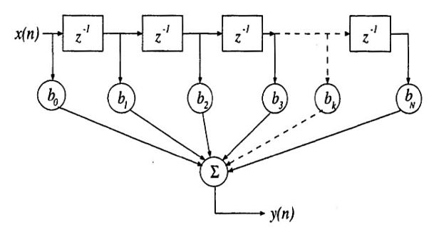
Fig: SFG of moving average filter of order N

Increased smoothing may be achieved by averaging signal samples over longer time windows, at the expense of increased filter delay. If the signal samples over a window of eight samples are averaged, we get the output as

The transfer function of filter becomes

The 8-point MA filter can be written as

The recursive form as above clearly depicts the integration aspect of the filter. The transfer function of this expression is easily derived to be

Techniques for Removal of Electrode Motion Artifacts

One of the widely used techniques for removing the electrode motion artifacts is based on adaptive filters. The general structure of an adaptive filter for noise cancelling utilized in this paper requires two inputs, called the primary and the reference signal. The former is the d(t) = s(t) + n1 (t) where s(t) is an ECG signal and n1(t) is an additive noise. The noise and the signal are assumed to be uncorrelated. The second input is a noise u(t) correlated in some way with n1 (t) but coming from another source. The adaptive filter coefficients wk are updated as new samples of the input signals are acquired. The learning rule for coefficients modification is based on minimization, in the mean square sense, of the error signal e(t) = d(t) − y(t) where y(t) is the output of the adaptive filter. A block diagram of the general structure of noise cancelling adaptive filtering is shown in figure. The two most widely used adaptive filtering algorithms are the Least Mean Square (LMS) and the Recursive Least Square (RLS).

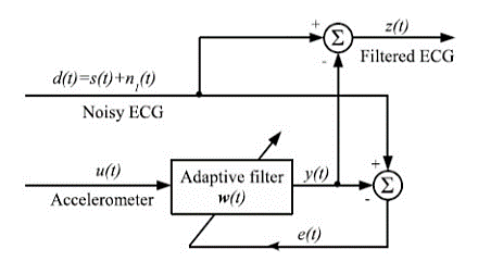
Fig: Block diagram of adaptive filtering scheme

Q16) What is digital image processing? How image is digitalised?

An image is denoted by a two dimensional function of the form f{x, y}. The value or amplitude of ‘f’ at spatial coordinates {x,y} is a positive scalar quantity whose physical meaning is determined by the source of the image. When an image is generated by a physical process, its values are proportional to energy radiated by a physical source. As a consequence, f(x,y) must be nonzero and finite; that is 0 <f(x,y) <∞

The function f(x,y) may be characterized by two components-

· The amount of the source illumination incident on the scene being viewed.

· The amount of the source illumination reflected back by the objects in the scene

These are called illumination and reflectance components and are denoted by i(x,y) and r(x,y) respectively. The functions combine as a product to form f(x,y)

We call the intensity of a monochrome image at any coordinate (x,y) the gray level of the image at that point l= f (x, y) , Lmin ≤ l ≤ Lmax

Lmin is to be positive and Lmax must be finite

Lmin = imin rmin

Lmax = imax rmax

The interval [Lmin, Lmax] is called gray scale. Common practice is to shift this interval numerically to the interval [0, L-l] where l=0 is considered black and l= L-1 is considered white on the gray scale. All intermediate values are shades of gray varying from black to white.

Image Digitization

To create a digital image, we need to convert the continuous sensed data into digital from.

This involves two processes – sampling and quantization. An image may be continuous

With respect to the x and y coordinates and also in amplitude. To convert it into digital form we have to sample the function in both coordinates and in amplitudes.

• Digitalizing the coordinate values is called sampling
• Digitalizing the amplitude values is called quantization

There is a continuous image along the line segment AB. To sample this function, we take equally spaced samples along line AB. The location of each sample is given by a vertical tick back (mark) in the bottom part. The samples are shown as block squares superimposed on function the set of these discrete locations gives the sampled function.

In order to form a digital image, the gray level values must also be converted (quantized) into discrete quantities. So we divide the gray level scale into eight discrete levels ranging from black to white. The vertical tick mark assign the specific value assigned to each of the eight level values.

The continuous gray levels are quantized simply by assigning one of the eight discrete gray levels to each sample. The assignment it made depending on the vertical proximity of a simple to a vertical tick mark.

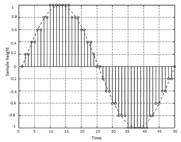
Starting at the top of the image and covering out this procedure line by line produces a two-dimensional digital image.

A digital image f[m,n] described in a 2D discrete space is derived from an analog image f(x,y) in a 2D continuous space through a sampling process that is frequently referred to as digitization. Some basic definitions associated with the digital image are described.

The 2D continuous image f(x,y) is divided into N rows and M columns. The intersection of a row and a column is termed a pixel. The value assigned to the integer coordinates [m,n] with {m=0,1,2,..., M-1}and{n=0,1,2,...,N-1}is f[m, n]. In fact, in most cases f(x,y) is actually a function of many variables including depth (d), color(μ) and time (t).

Q17) Explain how pixels are represented mathematically in digital image?

A17) The result of sampling and quantization is matrix of real numbers. Assume that an image f(x,y) is sampled so that the resulting digital image has M rows and N Columns. The values of the coordinates (x,y) now become discrete quantities thus the value of the coordinates at origin become (x,y) =(0,0) The next Coordinates value along the first signify the image along the first row. It does not mean that these are the actual values of physical coordinates when the image was sampled. Thus, the right side of the matrix represents a digital element, pixel or pel. The matrix can be represented in the following form as well.

The sampling process may be viewed as partitioning the x-y plane into a grid with the coordinates of the center of each grid being a pair of elements from the Cartesian products Z2 which is the set of all ordered pair of elements (Zi, Zj) with Zi and Zj being integers from Z.

Hence f(x,y) is a digital image if gray level (that is, a real number from the set of real number R) to each distinct pair of coordinates (x,y). This functional assignment is the quantization process. If the gray levels are also integers, Z replaces R, and a digital image become a 2D function whose coordinates and the amplitude value are integers.

Due to processing storage and hardware consideration, the number of gray levels typically is an integer power of 2. L=2K

Then, the number b, of bits required to store a digital image is

B=M *N* K

When M=N The equation become b=N2*K

When an image can have 2k gray levels, it is referred to as “k- bit”. An image with 256 possible gray levels is called an “8-bit image (because 256=28).

Q18) Write short note on special resolution?

A18) There are different definitions of spatial resolution but in a general and practical sense, it can be referred to as the size of each pixel. It is commonly measured in units of distance, i.e. cm or m. In other words, spatial resolution is a measure of the sensor’s ability to capture closely spaced objects on the ground and their discrimination as separate objects. Spatial resolution of a data depends on altitude of the platform used to record the data and sensor parameters. Relationship of spatial resolution with altitude can be understood with the following example. You can compare an astronaut on-board a space shuttle looking at the Earth to what he/she can see from an airplane. The astronaut might see a whole province or country at a single glance but will not Image Resolutions be able to distinguish individual houses. However, he/she will be able to see individual houses or vehicles while flying over a city or town. By comparing these two instances you will have better understanding of the concept of spatial resolution. This can be further elaborated by considering an example shown in Figure below.

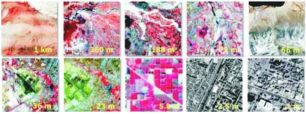
Fig: Spatial variations of remote sensing data.

Suppose you are looking at a forested hillside from a certain distance. What you see is the presence of the continuous forest; however from a great distance you do not see individual trees. As you go closer, eventually the trees, which may differ in size, shape, and species, become distinct as individuals. As you draw much nearer, you start to see individual leaves (Fig. Below). You can carry this even further, through leaf macro-structure, then recognition of cells, and with further higher spatial resolutions individual constituent atoms and finally subatomic components can be done.

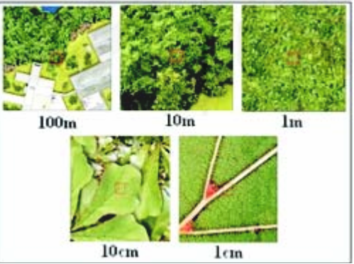
Fig: Understanding concept of spatial resolution

The details of features in an image are dependent on the spatial resolution of the sensor and refer to the size of the smallest possible feature that can be detected. Spatial resolution depends primarily on the Instantaneous Field of View (IFOV) (Fig.A) of the sensors which refers to the size of the smallest possible feature that can be detected by each sampling unit of the sensor. Usually, people think of resolution as spatial resolution, i.e. the fineness of the spatial detail visible in an image. The most commonly quoted quantity of the IFOV is the angle subtended by the geometrical projection of single detector element to the Earth’s surface.

Remote sensing instrument is located on a sub-orbital or satellite platform, where è of IFOV, is the angular field of view of the sensor (Fig. Below B). The segment of the ground surface measured within the IFOV is normally a circle of diameter D given by

D = è* H ………………...(1)

Where, D = diameter of the circular ground area viewed

H = flying height above the terrain, and

è = IFOV of the system (expressed in radians).

The ground segment sensed at any instant is called ground resolution element or resolution cell.

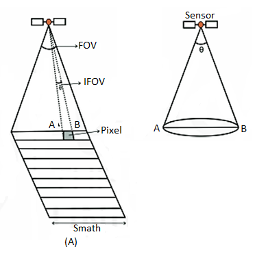
Fig: Schematics showing (A) relationship of IFOV and FOV and (B) concept of IFOV

Spatial resolution of remote sensing system is influenced by the swath width. Spatial resolution and swath width determine the degree of detail that is revealed by the sensors and the area of coverage. Remote sensing sensors are generally categorised into coarse, intermediate and high spatial resolution sensors based on their spatial resolution. Sensors having coarse resolution provide much less detail than the high spatial resolution sensors. Because of the level of details, the sensors provide, they are used for mapping at different scales. High spatial resolution sensors are used for large scale mapping (small area mapping) whereas coarse spatial resolution data are used for regional, national and global scale mapping.

Q19) What is temporal resolution?

A19) In addition to spatial, spectral and radiometric resolution, it is also important to consider the concept of temporal resolution in a remote sensing system. One of the advantages of remote sensing is its ability to observe a part of the Earth (scene) at regular intervals. The interval at which a given scene can be imaged is called temporal resolution. Temporal resolution is usually expressed in days. For instance, IRS-1A has 22 days temporal resolution, meaning it can acquire image of a particular area in 22 days interval, respectively.

Low temporal resolution refers to infrequent repeat coverage whereas high temporal resolution refers to frequent repeat coverage. Temporal resolution is useful for agricultural application (Fig. Below) or natural disasters like flooding (Fig. Below) when you would like to re-visit the same location within every few days. The requirement of temporal resolution varies with different applications. For example, to monitor agricultural activity, image interval of 10 days would be required, but intervals of one year would be appropriate to monitor urban growth patterns.

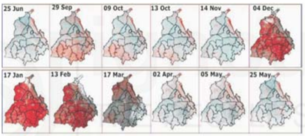
Fig: Temporal variations of remote sensing data used to monitor changes in agriculture, showing crop conditions in different months

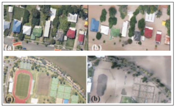
Fig: Showing the importance of temporal resolution.

Approximately 0945 h and 1030 h local sun time, respectively. However, this is subject to slight variation due to orbital perturbations. Both satellites pass overhead earlier in the day north of the equator and later to the south. The cross-track width of the imaging strip is an important parameter in deciding temporal resolution.

Q20) How convolution is performed in 2D for extraction? Also explain with an example how padding of zero is used in this process?

A20) When convolution between two signals which are spanning around mutually perpendicular dimensions is called as 2D convolution. The convolution is similar to 1D convolution where it is done by multiplying and accumulating the instantaneous values of oversampling samples which are corresponding to the two input signals, out of which one is flipped. This can be understood with help of one example.

Let the below matrix x be of the original image and h represent the kernel.

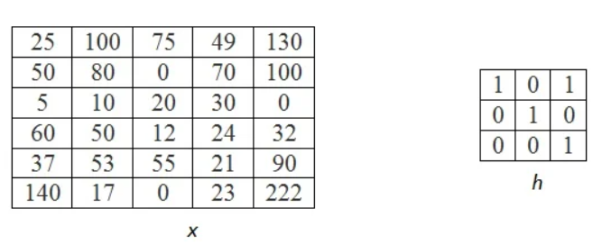
Step 1

In this firstly the rows are converted to columns, and then again rows are flipped along the columns. We can also say that (i,j)th element of original kernel become the (j,i)th element of new matrix.

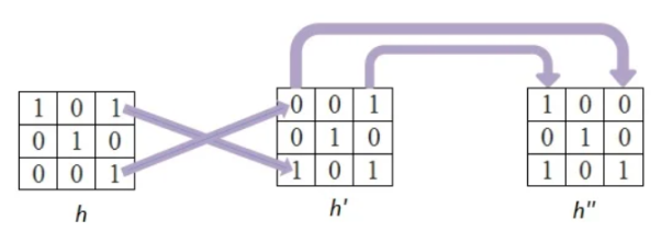
Step 2

Next the inverted kernels are overlapped over the image pixel by pixel. The product of mutually overlapping pixels is calculated and their sums are found. This becomes the value of output pixel for that particular location. Where there is no overlapping pixel, it is assumed to be 0.

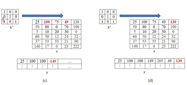
The above process is now shown in detail. When pixel of kernel at bottom right falls on first pixel of the image matrix at the top left. The value 25x1 =25 becomes the first pixel value of the output image.

Now the two value of kernel matrix (0,1) in the same row overlap with two pixels of the image (25, 100). The output pixel will be (25x0+100x1) = 100.

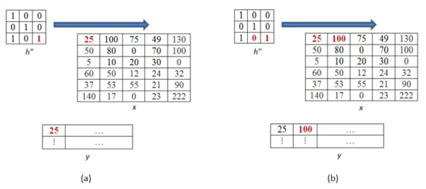
Further continuing same process, we get the values of the output pixels for each pixel. The fourth and seventh output pixel matrix are shown below.

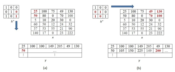
When we move vertically down by a single pixel then the first overlap is shown below. The value of output pixel is obtained by MAC [25x0+50x1] =50. Further we keep moving until we find overlap between all values of kernel and image matrices. For example, the sixth output pixel value will be [49x0 +130x1+70x1+100x0] =200 shown below.

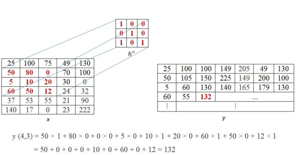
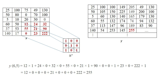
This process of moving one step down followed by horizontal scanning has to be continued until the last row of the image matrix. Three random examples concerned with the pixel outputs at the locations (4,3), (6,5) and (8,6) are shown in Figure below.

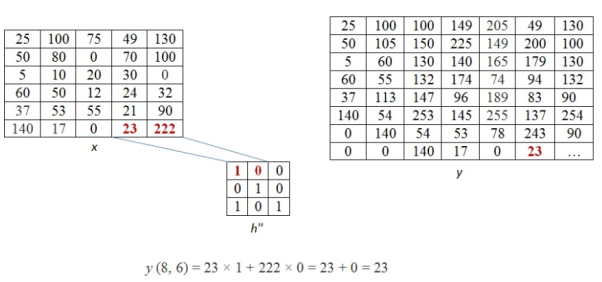
The value of the final output matrix will be

Padding Zero

The convolution for 2D is given by

X: input image matrix

H: kernel matrix

Y: Output image

i,j: indices of image matrix

Let us suppose 3x3 kernel convolve then m and n range from -1 to 1. The expansion will now be

y[i,j]=

y[i,j]=h[−1,−1]⋅x[i+1,j+1]+h[−1,0]⋅x[i+1,j]+h[−1,1]⋅x[i+1,j−1]+h[0,−1]⋅x[i,j+1]+h[0,0]⋅x[i,j]+h[0,1]⋅x[i,j−1]+h[1,−1]⋅x[i−1,j+1]+h[1,0]⋅x[i−1,j]+h[1,1]⋅x[i−1,j−1]

From above equation we see that in order to find every output pixel nine multiplications are required. The result obtained by the summation of nine product terms can be equal to the product of a single term if the collective effect of the other eight product terms equalizes to zero. One such way is the case in which each product of the other eight terms evaluates, themselves to be zero. In the context of our example, this means, all the product terms corresponding to the non-overlapping (between image and the kernel) pixels must become zero in order to make the results of formula-computation equal to that of graphical-computation.

If at least one of the factors involved in multiplication is zero, then the resulting product is also zero. By this analogy, we can state that, in our example, we need to have a zero-valued image-pixel corresponding to each non-overlapping pixels of the kernel matrix.

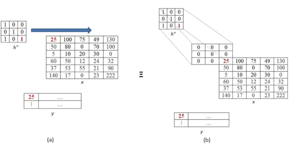
The process of adding zeros is called zero padding. It is done in all the places where the image pixel and kernel pixel do not overlap.

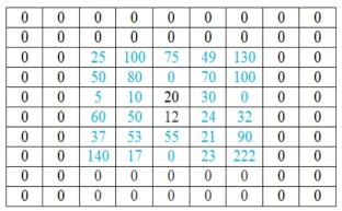
The number of rows or column to be padded with 0 are calculated as number of rows or column in kernel-1.