UNIT 2

Plane Stress and Plane Strain Problems

Q1) Explain Plane stresses?

A1) A plane stress problem is taken to be one in which σzz is zero. As stated above, cases where a uniform stress is applied to the plane surfaces can easily be reduced to this condition by application of a suitable σzz stress of opposite sign. Shear components in the Z direction must also be zero.

i.e.

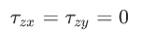
Under these conditions the stress equations of equilibrium in cartesian coordinates reduce to

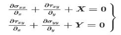
The following stress and strain relationships then apply:

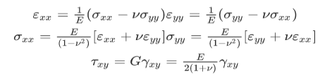
Plane stress systems are often referred to as two-dimensional or bi-axial stress systems, a typical example of which is the case of thin plates loaded at their edges with forces applied in the plane of the plate.

Q2) Introduce Airy Stress Functions?

A2) The use of Airy Stress Functions is a powerful technique for solving 2-D equilibrium problems. They are covered here because the approach was used by several researchers in the mid 1900's to develop analytical solutions to linear elastic problems involving cracks. The curious fact about Airy stress functions is that their use typically leads one to obtain a solution first, and then the next step is to determine what the actual problem to which the solution applies is. It's as if the answer comes before the question.

Q3) What is Equilibrium?

A3) The story of Airy stress functions begins with the concept of equilibrium. Everyone knows that ∑F=ma, and if the object is in equilibrium, then a=0a=0 and ∑F=0.

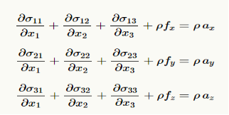
The governing differential equation for equilibrium expresses ∑F=ma  in terms of derivatives of the stress tensor as

∇⋅σ + ρf =ρa

Where

σ is the stress tensor

ρ is density

f is the body force vector

a is the acceleration vector

A derivation of the equilibrium equation is given below. The complete set of equations Is

Q4) Explain the Airy solution in rectangular coordinates?

A4) The Airy function procedure can then be summarized as follows:

Begin by finding a scalar function  (known as the Airy potential) which satisfies:

Where

In addition  must satisfy the following traction boundary conditions on the surface of the solid

Where  (n1, n2) are the components of a unit vector normal to the boundary.

2.  Given  the stress field within the region of interest can be calculated from the formulas

If the strains are needed, they may be computed from the stresses using the elastic stressstrain relations.

4.  If the displacement field is needed, it may be computed by integrating the strains,.  An example (in polar coordinates) is given in below.

Although it is easier to solve for  than it is to solve for stress directly, this is still not a trivial exercise.  Usually, one guesses a suitable form for  , as illustrated.  This may seem highly unsatisfactory, but remember that we are essentially integrating a system of PDEs.  The general procedure to evaluate any integral is to guess a solution, differentiate it, and see if the guess was correct. 

Q5) Explain 2D Line load acting parallel to the surface of an infinite solid?

A5) Similarly, the stress fields due to a line load magnitude P per unit out-of-plane length acting tangent to the surface of a homogeneous, isotropic half-space can be generated from the Airy function

The formulas in the preceding section yield

The method outlined in the preceding section can be used to calculate the displacements. The procedure gives

To within an arbitrary rigid motion

The stresses and displacements in the  basis are

Q6) Explain arbitrary pressure acting on a flat surface?

A6) The principle of superposition can be used to extend the point force solutions to arbitrary pressures acting on a surface. For example, we can find the (plane strain) solution for uniform pressure acting on the strip of width 2a on the surface of a half-space by distributing the point force solution appropriately.

Distributing point forces with magnitude    over the loaded region shows that

Q7) Explain Uniform normal pressure acting on a strip?

A7) For the particular case of a uniform pressure, the integrals can be evaluated to show that

Where  and 

Q8) Explain stresses near the tip of a crack?

A8) Consider an infinite solid, which contains a semi-infinite crack on the (x1, x3) plane. Suppose that the solid deforms in plane strain and is subjected to bounded stress at infinity.  The stress field near the tip of the crack can be derived from the Airy function.

Here KI and KII are two constants, known as mode I and mode II stress intensity factors, respectively.  They quantify the magnitudes of the stresses near the crack tip, as shown below. The stresses can be calculated as

Equivalent expressions in rectangular coordinates are

While the displacements can be calculated by integrating the strains, with the result

Note that this displacement field is valid for plane strain deformation only.

Observe that the stress intensity factor has the bizarre units of .

Q9) Discuss Airy function solution to the end loaded cantilever?

A9) Consider a cantilever beam, with length L, height 2a and out-of-plane thickness b, as shown in the figure. The beam is made from an isotropic linear elastic solid with Young’s modulus  E and Poisson ratio v The top and bottom of the beam  are traction free, the left hand end is subjected to a resultant force P, and the right hand end is clamped.  Assume that b<<a, so that a state of plane stress is developed in the beam. An approximate solution to the stress in the beam can be calculated from the Airy function

You can easily show that this function satisfies the governing equation for the Airy function. The stresses follow as

To see that this solution satisfies the boundary conditions, note that

The top and bottom surfaces of the beam  are traction free (  ) since the normal is in the  e2 direction on these surfaces, this requires that.  The stress field clearly satisfies this condition.

2.  The plane stress assumption automatically satisfies boundary conditions on 

3.   The traction boundary condition on the left hand end of the beam (x1=0) was not specified in detail: instead, we only required that the resultant of the traction acting on the surface is  –Pe2 The normal to the surface at the left hand end of the beam is in the  -e1 direction, so the traction vector is

The resultant force can be calculated by integrating the traction over the end of the beam:

The stresses thus satisfy the boundary condition.  Note that by Saint-Venant’s principle, other distributions of traction with the same resultant will induce the same stresses sufficiently far (x1>3a) from the end of the beam.

4. The boundary conditions on the right hand end of the beam are not satisfied exactly.  The exact solution should satisfy both  u1=0 and  u2=0 on x1=L The displacement field corresponding to the stress distribution was calculated in the example problem in Sect 2.1.20, where we found that

Where  c,d,w are constants that may be selected to satisfy the boundary condition as far as possible.  We can satisfy u1=0 and  u2=0 at some, but not all, points on x1=L The choice is arbitrary.  Usually the boundary condition is approximated by requiring   at  x1=L,  x2=0 This gives C=0, d=-PL3/2Ea3b and W= 3PL2/4Ea3b By Saint-Venant’s principle, applying other boundary conditions (including the exact boundary condition) will not influence the stresses and displacements sufficiently far from the end.

Q10) Write important airy governing equations?

A10) Demonstration that the Airy solution satisfies the governing equations

Recall that to solve a linear elasticity problem, we need to satisfy the following equations:

1 Displacementstrain relation          

2 Stressstrain relation

3 Equilibrium Equations