UNIT 3
Correlation and Regression
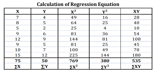
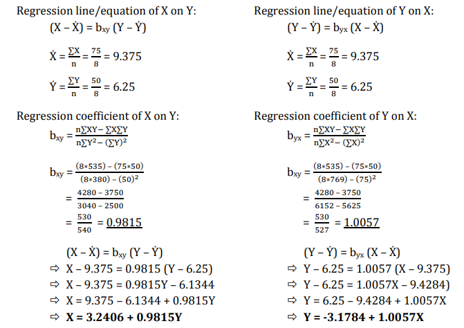
Q1) From the following data obtain the two regression lines:
Capital Employed (Rs. in lakh): 7 8 5 9 12 9 10 15
Sales Volume (Rs. in lakh): 4 5 2 6 9 5 7 12
A1)
Q2) After investigation it has been found the demand for automobiles in a city depends mainly, if not entirely, upon the number of families residing in that city. Below are the given figures for the sales of automobiles in the five cities for the year 2019 and the number of families residing in those cities.
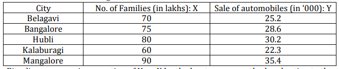
Fit a linear regression equation of Y on X by the least square method and estimate the sales for the year 2020 for the city Belagavi which is estimated to have 100 lakh families assuming that the same relationship holds true.
A2)
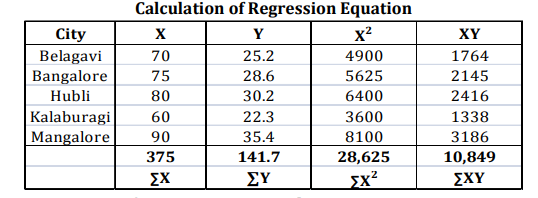
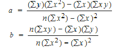
Regression equation of Y on X: Y = a + bX
The two normal equations are:
∑Y = Na + b∑X
∑XY = a∑X + b∑X2
Substituting the values in above normal equations, we get
141.7 = 5a + 375b ..... (i)
10849= 375a + 28625b ..... (ii)
Let us solve these equations (i) and (ii) by simultaneous equation method
Multiply equation (i) by 75 we get 10627.5 = 375a + 28125b
Now rewriting these equations:
10627.5 = 375a + 28125b
10849 = 375a + 28625b
(-) (-) (-) .
-221.5 = -500b
Therefore now we have -221.5 = -500b, this can rewritten as 500b = 221.5
Now, b = 221.5/500 = 0.443
Substituting the value of b in equation (i), we get
141.7 = 5a + (375 * 0.443)
141.7 = 5a + 166.125
5a = 141.7 - 166.125
5a = -24.425
a = -24.425/5
a = -4.885
Thus we got the values of a = -4.885 and b = 0.443
Hence, the required regression equation of Y on X:
Y = a + bX => Y = -4.885 + 0.443X
Estimated sales of automobiles (Y) in city Belagavi for the year 2020, where number of families (X) are 100(in lakhs):
Y = -4.885 + 0.443X
Y = -4.885 + (0.443 * 100)
Y = -4.885 + 44.3
Y = 39.415 (‘000)
Means sales of automobiles would be 39,415 when number of families are 100,00,000
Q3) Given below are five observation collected in simple regression. Calculate the intercept, slope and write down the estimated regression equation
X | Y |
2 | 7 |
4 | 5 |
6 | 4 |
8 | 2 |
10 | 1 |
A3)
X | Y | X2 | y2 | xy |
2 | 7 | 4 | 49 | 14 |
4 | 5 | 16 | 25 | 20 |
6 | 4 | 36 | 16 | 24 |
8 | 2 | 64 | 4 | 16 |
10 | 1 | 100 | 1 | 10 |
30 | 19 | 220 | 95 | 84 |
To find a and b, use the following equation
Find a:
((19 × 220) – ((30 × 84)) / 5 (220) – 900)
1660/ 200
=8.3
Find b:
(5(84) – (30 × 19)) / (5 (220) – 900)
-150 / 200
= -0.75
y’ = a + bx
y’ = 8.3 + (-0.75)x
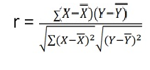
Q4) Calculate Karl Pearson’s Coefficient of Correlation
X | 28 | 45 | 40 | 38 | 35 | 33 | 40 | 32 | 36 | 33 |
Y | 23 | 34 | 33 | 34 | 30 | 26 | 28 | 31 | 36 | 35 |
A4)
X | Y |
|
|
|
| |
28 | 23 | -8 | 64 | -8.0 | 64.0 | 64.0 |
45 | 34 | 9 | 81 | 3.0 | 9.0 | 27.0 |
40 | 33 | 4 | 16 | 2.0 | 4.0 | 8.0 |
38 | 34 | 2 | 4 | 3.0 | 9.0 | 6.0 |
35 | 30 | -1 | 1 | -1.0 | 1.0 | 1.0 |
33 | 26 | -3 | 9 | -5.0 | 25.0 | 15.0 |
40 | 28 | 4 | 16 | -3 | 9 | -12.0 |
32 | 31 | -4 | 16 | 0 | 0 | 0.0 |
36 | 36 | 0 | 0 | 5 | 25 | 0.0 |
33 | 35 | -3 | 9 | 4 | 16 | -12 |
360 | 310 | 0 | 216 | 0 | 162 | 97 |


 X = 360/10 = 36
Y = 310/10 = 31
r = 97/(√216 √162 = 0.51
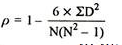
Q5) Calculates spearman rank correlation
X | 10 | 15 | 11 | 14 | 16 | 20 | 10 | 8 | 7 | 9 |
Y | 16 | 16 | 24 | 18 | 22 | 24 | 14 | 10 | 12 | 14 |
A5)
X | Y | Rank X | Rank Y | D | d2 |
10 | 16 | 6.5 | 5.5 | 1 | 1 |
15 | 16 | 3 | 5.5 | -2.5 | 6.25 |
11 | 24 | 5 | 1.5 | 3.5 | 12.25 |
14 | 18 | 4 | 4 | 0 | 0 |
16 | 22 | 2 | 3 | -1 | 1 |
20 | 24 | 1 | 1.5 | -0.5 | 0.25 |
10 | 14 | 6.5 | 7.5 | -1 | 1 |
8 | 10 | 9 | 10 | -1 | 1 |
7 | 12 | 10 | 9 | 1 | 1 |
9 | 14 | 8 | 7.5 | 0.5 | 0.25 |
|
|
|
|
| 24 |
R = 1 – (6*24)/10(102 – 1) = 0.85
The correlation between X and Y is positive and very high.
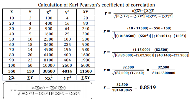
Q6) Find Karl Pearson’s coefficient of correlation between capital employed and profit obtained from the following data.
A6)
Let us assume that capital employed is variable X and profit is variable Y.

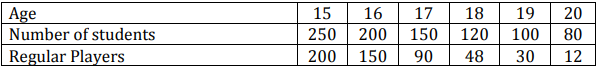
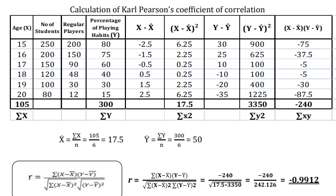
Q7) Find the correlation coefficient between age and playing habits of the following students using Karl Pearson’s coefficient of correlation method
A7)
To find the correlation between age and playing habits of the students, we need to compute the percentages of students who are having the playing habit.
Percentage of playing habits = No. of Regular Players / Total No. of Students * 100
Now, let us assume that ages of the students are variable X and percentages of playing habits are variable Y.
Interpretation: From the above calculation it is very clear that there is high degree of negative correlation i.e. r = -0.9912, between the two variables of age and playing habits. i.e. Playing habits among students decreases when their age increases.
Q8) Find out spearman’s coefficient of correlation between the two kinds of assessment of graduate students’ performance in a college.
A8)
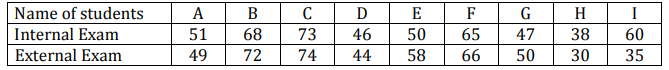
Interpretation: From the above calculation it is very clear that there is high degree of positive correlation i.e. R = 0.7833, between two exams. It means there is a high degree of positive correlation between the internal exam and external exam of the students.
Q9) Compute Pearson’s coefficient of correlation between advertisement cost and sales as per the data given below:
Advertisement cost | 39 | 65 | 62 | 90 | 82 | 75 | 25 | 98 | 36 | 78 |
sales | 47 | 53 | 58 | 86 | 62 | 68 | 60 | 91 | 51 | 84 |
A9)
X | Y |
|
|
|
| |
39 | 47 | -26 | 676 | -19 | 361 | 494 |
65 | 53 | 0 | 0 | -13 | 169 | 0 |
62 | 58 | -3 | 9 | -8 | 64 | 24 |
90 | 86 | 25 | 625 | 20 | 400 | 500 |
82 | 62 | 17 | 289 | -4 | 16 | -68 |
75 | 68 | 10 | 100 | 2 | 4 | 20 |
25 | 60 | -40 | 1600 | -6 | 36 | 240 |
98 | 91 | 33 | 1089 | 25 | 625 | 825 |
36 | 51 | -29 | 841 | -15 | 225 | 435 |
78 | 84 | 13 | 169 | 18 | 324 | 234 |
650 | 660 |
| 5398 |
| 2224 | 2704 |
|
|
|
|
|
|
|


r = (2704)/√5398 √2224 = (2704)/(73.2*47.15) = 0.78
Thus Correlation coefficient is positively correlated
Q10) Compute correlation coefficient from the following data
Hours of sleep (X) | Test scores (Y) |
8 | 81 |
8 | 80 |
6 | 75 |
5 | 65 |
7 | 91 |
6 | 80 |
A10)
X | Y |
|
|
|
| |
8 | 81 | 1.3 | 1.8 | 2.3 | 5.4 | 3.1 |
8 | 80 | 1.3 | 1.8 | 1.3 | 1.8 | 1.8 |
6 | 75 | -0.7 | 0.4 | -3.7 | 13.4 | 2.4 |
5 | 65 | -1.7 | 2.8 | -13.7 | 186.8 | 22.8 |
7 | 91 | 0.3 | 0.1 | 12.3 | 152.1 | 4.1 |
6 | 80 | -0.7 | 0.4 | 1.3 | 1.8 | -0.9 |
40 | 472 |
| 7 |
| 361 | 33 |


X = 40/6 =6.7

Y = 472/6 = 78.7

r = (33)/√7 √361 = (33)/(2.64*19) = 0.66
Thus Correlation coefficient is positively correlated


