UNIT 2

Searching and Sorting

1. Explain Sequential Search

This is the traditional technique for searching an element in a collection of elements. In this type of search, all the elements of the list are traversed one by one to find if the element is present in the list or not. One example of such an algorithm is a linear search. This is a very simple and basic algorithm. Suppose ARR is an array of n elements, and we need to find location LOC of element ITEM in ARR. For this, LOC is assigned to -1 which indicates that ITEM is not present in ARR. While comparing ITEM with data at each location of ARR, and once ITEM == ARR[N], LOC is updated with location N+1. Hence we found the ITEM in ARR.

Algorithm:

LSEARCH(ARR, N, ITEM, LOC) Here ARR Is the array of N number of elements, ITEM holds the value we need to search in the array and algorithm returns LOC, the location where ITEM is present in the ARR. Initially, we have to set LOC = -1.

1. Set LOC = -1,i=1
2. Repeat while DATA[i] != ITEM:
i=i+1
3. If i=N+1 ,then Set LOC =0
Else LOC = N+1
4. Exit.

Let’s say, below is the ARR with 10 elements. And we need to find whether ITEM= 18 is present in this array or not. 

In the start, LOC =-1

Step 1: ITEM != 77 thus we move to next element.

Step 2: ITEM != 56 thus we move to next element.

Step 3: ITEM != 14 thus we move to next element.

Step 4: ITEM != 7 thus we move to the next element.

Step 5: Hence ITEM == ARR[4] thus LOC updated to 5.

Complexity of Sequential Search

Here are the complexities of the linear search given below.

Space complexity

As linear search algorithm does not use any extra space thus its space complexity = O(n) for an array of n number of elements.

Time Complexity

• Worst case complexity: O(n) – This case occurs when the element to search is not present in the array.
• Best case complexity: O(1) – This case occurs when the first element is the element to be searched.
• Average complexity: O(n) – This means when an element is present somewhere in the middle of the array.

2.     Explain Binary Search

This is a technique to search an element in the list using the divide and conquer technique. This type of technique is used in the case of sorted lists. Instead of searching an element one by one in the list, it directly goes to the middle element of the list and divides the array into 2 parts, and decides element lies in which sub-array does the element exist.

Suppose ARR is an array with sorted n number of elements present in increasing order. With every step of this algorithm, the searching is confined within BEG and END, which are the beginning and ending index of sub-arrays. The index MID defines the middle index of the array where,

MID = INT(beg + end )/2

And then, it needs to be checked if ITEM < ARR[N} where ITEM is the element that we need to search in ARR.

• If ITEM = ARR[MID] then LOC = MID and exit .
• If ITEM < ARR[MID} then ITEM can appear in the left sub-array, then BEG will be the same and END = MID -1 and repeat.
• If ITEM > ARR[MID] then ITEM can appear in the right subarray then BEG = MID+1 and END will be the same and repeat.

After this MID is again calculated for respective sub-arrays. In case we didn’t find the ITEM, the algorithm returns -1 otherwise LOC = MID.

Algorithm:

BSEARCH(ARR, LB, UB, ITEM, LOC) Here, ARR is a sorted list of elements, with LB and UB are lower and upper bounds for the array. ITEM needs to be searched in the array and algorithm returns location LOC, index at which ITEM is present else return -1.

1. Set BEG = LB, END = UB and MID = INT([BEG+END]/2)
2. Repeat step 3 and 4 while BEG <= END and ARR[MID] != ITEM
3. IF ITEM< ARR[MID] then:
Set END = MID-1
Else:
Set BEG = MID+1
4. Set MID = INT(BEG+END)/2
5. IF ARR[MID] = ITEM then:
Set LOC = MID
Else:
Set LOC = NULL
6. Exit.

Let’s say here, ITEM = 62

BEG = 1 and END =9 Hence MID = (1+9)/2 = 5
ARR[MID] = 52

Step 1: ARR[MID] < ITEM : thus END =9 and BEG = MID +1 = 6. Thus our new sub-array is,

Step 2: Now BEG =6 and END =9 thus MID = INT([6+9]/2)= 6
NOW ARR[6] =ITEM. Thus LOC = MID
Thus LOC = 6

Complexity of Binary Search

Here are the complexities of the binary search given below.

• Worst Case: O(nlogn)
• Best Case: O(1)
• Average Case: O(nlogn)

Conclusion

Searching refers to finding the location of one element in the array of n elements. There are 2 types of search linear and binary Search, Linear search algorithm is very simple and has O(n) of complexity whereas Binary Search is a very fast searching algorithm having the complexity of (logn) but can only be used in case of the sorted list of elements. In case the size of the array is large, it is preferable to use binary search instead of linear search. Binary search is used in many searching data structures. In the case of mid-size arrays, the linear search algorithm is more preferred.

3.    Explain Sorting Techniques

Sorting refers to arranging data in a particular format. Sorting algorithm specifies the way to arrange data in a particular order. Most common orders are in numerical or lexicographical order.

The importance of sorting lies in the fact that data searching can be optimized to a very high level, if data is stored in a sorted manner. Sorting is also used to represent data in more readable formats. Following are some of the examples of sorting in real-life scenarios −

• Telephone Directory − The telephone directory stores the telephone numbers of people sorted by their names, so that the names can be searched easily.
• Dictionary − The dictionary stores words in an alphabetical order so that searching of any word becomes easy.

In-place Sorting and Not-in-place Sorting

Sorting algorithms may require some extra space for comparison and temporary storage of few data elements. These algorithms do not require any extra space and sorting is said to happen in-place, or for example, within the array itself. This is called in-place sorting. Bubble sort is an example of in-place sorting.

However, in some sorting algorithms, the program requires space which is more than or equal to the elements being sorted. Sorting which uses equal or more space is called not-in-place sorting. Merge-sort is an example of not-in-place sorting.

Stable and Not Stable Sorting

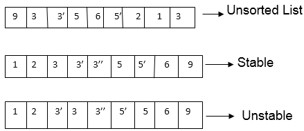
If a sorting algorithm, after sorting the contents, does not change the sequence of similar content in which they appear, it is called stable sorting.

If a sorting algorithm, after sorting the contents, changes the sequence of similar content in which they appear, it is called unstable sorting.

Stability of an algorithm matters when we wish to maintain the sequence of original elements, like in a tuple for example.

Adaptive and Non-Adaptive Sorting Algorithm

A sorting algorithm is said to be adaptive, if it takes advantage of already 'sorted' elements in the list that is to be sorted. That is, while sorting if the source list has some element already sorted, adaptive algorithms will take this into account and will try not to re-order them.

A non-adaptive algorithm is one which does not take into account the elements which are already sorted. They try to force every single element to be re-ordered to confirm their sortedness.

Important Terms

Some terms are generally coined while discussing sorting techniques, here is a brief introduction to them −

Increasing Order

A sequence of values is said to be in increasing order, if the successive element is greater than the previous one. For example, 1, 3, 4, 6, 8, 9 are in increasing order, as every next element is greater than the previous element.

Decreasing Order

A sequence of values is said to be in decreasing order, if the successive element is less than the current one. For example, 9, 8, 6, 4, 3, 1 are in decreasing order, as every next element is less than the previous element.

Non-Increasing Order

A sequence of values is said to be in non-increasing order, if the successive element is less than or equal to its previous element in the sequence. This order occurs when the sequence contains duplicate values. For example, 9, 8, 6, 3, 3, 1 are in non-increasing order, as every next element is less than or equal to (in case of 3) but not greater than any previous element.

Non-Decreasing Order

A sequence of values is said to be in non-decreasing order, if the successive element is greater than or equal to its previous element in the sequence. This order occurs when the sequence contains duplicate values. For example, 1, 3, 3, 6, 8, 9 are in non-decreasing order, as every next element is greater than or equal to (in case of 3) but not less than the previous one.

4.    Explain Sort stability

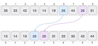
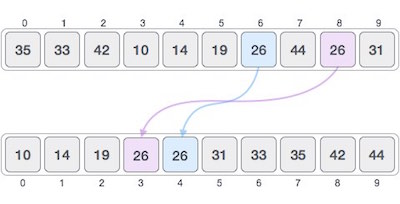
A sorting algorithm is said to be stable if two objects with equal keys appear in the same order in sorted output as they appear in the input unsorted array.

Some Sorting Algorithm is stable by nature like Insertion Sort, Merge Sort and Bubble Sort etc.

Sorting Algorithm is not stable like Quick Sort, Heap Sort etc.

Another Definition of Stable Sorting:

A Stable Sort is one which preserves the original order of input set, where the comparison algorithm does not distinguish between two or more items. A Stable Sort will guarantee that the original order of data having the same rank is preserved in the output.

In Place Sorting Algorithm:

1. An In-Place Sorting Algorithm directly modifies the list that is received as input instead of creating a new list that is then modified.
2. In this Sorting, a small amount of extra space it uses to manipulate the input set. In other Words, the output is placed in the correct position while the algorithm is still executing, which means that the input will be overwritten by the desired output on run-time.
3. In-Place, Sorting Algorithm updates input only through replacement or swapping of elements.
4. An algorithm which is not in-place is sometimes called not-in-Place or out of Place.
5. An Algorithm can only have a constant amount of extra space, counting everything including function call and Pointers, Usually; this space is O (log n).

Note:

1. Bubble sort, insertion sort, and selection sort are in-place sorting algorithms. Because only swapping of the element in the input array is required.
2. Bubble sort and insertion sort can be applying as stable algorithms but selection sort cannot (without significant modifications).
3. Merge sort is a stable algorithm but not an in-place algorithm. It requires extra array storage.
4. Quicksort is not stable but is an in-place algorithm.
5. Heap sort is an in-place algorithm but is not stable.

5. Explain Linear Search

Linear search is the simplest search algorithm and often called sequential search. In this type of searching, we simply traverse the list completely and match each element of the list with the item whose location is to be found. If the match found then location of the item is returned otherwise the algorithm return NULL.

Linear search is mostly used to search an unordered list in which the items are not sorted. The algorithm of linear search is given as follows.

Algorithm

• LINEAR_SEARCH(A, N, VAL)
• Step 1: [INITIALIZE] SET POS = -1
• Step 2: [INITIALIZE] SET I = 1
• Step 3: Repeat Step 4 while I<=N
• Step 4: IF A[I] = VAL
  SET POS = I
  PRINT POS
  Go to Step 6
  [END OF IF]
  SET I = I + 1
  [END OF LOOP]
• Step 5: IF POS = -1
  PRINT " VALUE IS NOT PRESENTIN THE ARRAY "
  [END OF IF]
• Step 6: EXIT

Complexity of algorithm

C Program

1. #include<stdio.h>   
2. Void main ()  
3. {  
4.    Int a[10] = {10, 23, 40, 1, 2, 0, 14, 13, 50, 9};  
5.    Int item, i,flag;  
6.    Printf("\nEnter Item which is to be searched\n");  
7.    Scanf("%d",&item);  
8.    For (i = 0; i< 10; i++)  
9.    {  
10.        If(a[i] == item)   
11.        {  
12.            Flag = i+1;  
13.            Break;  
14.        }   
15.        Else   
16.        Flag = 0;  
17.    }   
18.    If(flag != 0)  
19.    {  
20.        Printf("\nItem found at location %d\n",flag);  
21.    }  
22.    Else  
23.    {  
24.        Printf("\nItem not found\n");   
25.    }  
26. }   

Output:

Enter Item which is to be searched

20

Item not found

Enter Item which is to be searched

23

Item found at location 2

6.     Explain Binary Search

Binary search is the search technique which works efficiently on the sorted lists. Hence, in order to search an element into some list by using binary search technique, we must ensure that the list is sorted.

Binary search follows divide and conquer approach in which, the list is divided into two halves and the item is compared with the middle element of the list. If the match is found then, the location of middle element is returned otherwise, we search into either of the halves depending upon the result produced through the match.

Binary search algorithm is given below.

BINARY_SEARCH(A, lower_bound, upper_bound, VAL)

• Step 1: [INITIALIZE] SET BEG = lower_bound
  END = upper_bound, POS = - 1
• Step 2: Repeat Steps 3 and 4 while BEG <=END
• Step 3: SET MID = (BEG + END)/2
• Step 4: IF A[MID] = VAL
  SET POS = MID
  PRINT POS
  Go to Step 6
  ELSE IF A[MID] > VAL
  SET END = MID - 1
  ELSE
  SET BEG = MID + 1
  [END OF IF]
  [END OF LOOP]
• Step 5: IF POS = -1
  PRINT "VALUE IS NOT PRESENT IN THE ARRAY"
  [END OF IF]
• Step 6: EXIT

Complexity

Example

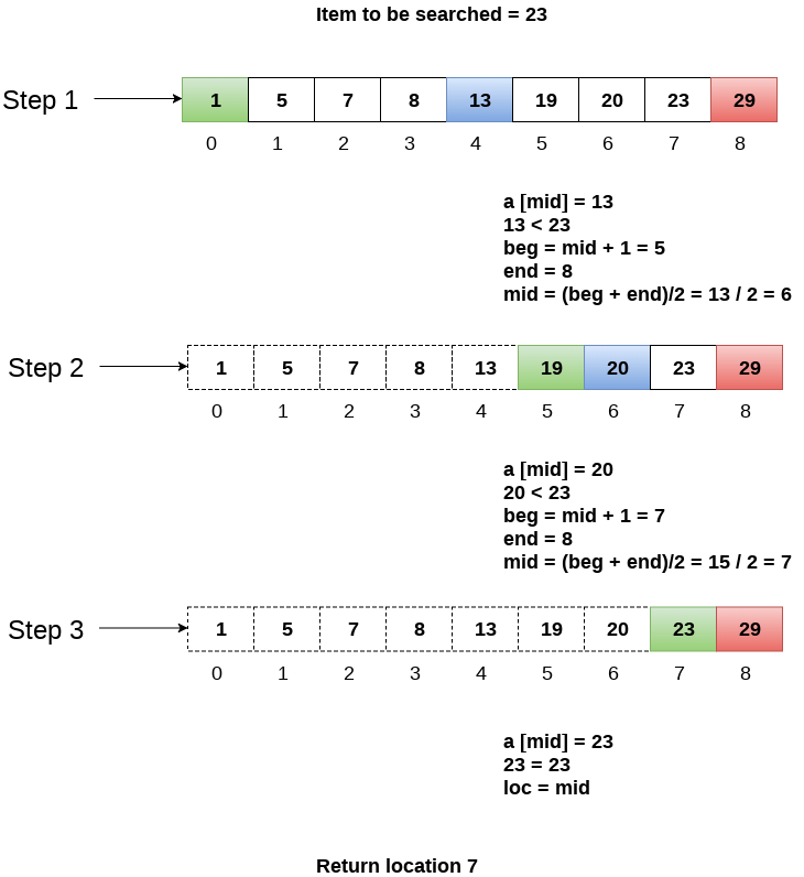
Let us consider an array arr = {1, 5, 7, 8, 13, 19, 20, 23, 29}. Find the location of the item 23 in the array.

In 1st step :

1. BEG = 0   
2. END = 8ron  
3. MID = 4   
4. a[mid] = a[4] = 13 < 23, therefore  

In Second step:

1. Beg = mid +1 = 5   
2. End = 8  
3. Mid = 13/2 = 6    
4. a[mid] = a[6] = 20 < 23, therefore;   

In third step:

1. Beg = mid + 1 = 7   
2. End = 8   
3. Mid = 15/2 = 7  
4. a[mid] = a[7]   
5. a[7] = 23 = item;   
6. Therefore, set location = mid;   
7. The location of the item will be 7.   

7.     Explain Binary Search Program using Recursion

C program

1. #include<stdio.h>  
2. Int binarySearch(int[], int, int, int);  
3. Void main ()  
4. {  
5.    Int arr[10] = {16, 19, 20, 23, 45, 56, 78, 90, 96, 100};  
6.    Int item, location=-1;   
7.    Printf("Enter the item which you want to search ");  
8.    Scanf("%d",&item);  
9.    Location = binarySearch(arr, 0, 9, item);  
10.    If(location != -1)   
11.    {  
12.        Printf("Item found at location %d",location);  
13.    }  
14.    Else  
15.    {  
16.        Printf("Item not found");  
17.    }  
18. }   
19. Int binarySearch(int a[], int beg, int end, int item)  
20. {  
21.    Int mid;  
22.    If(end >= beg)   
23.    {     
24.        Mid = (beg + end)/2;  
25.        If(a[mid] == item)  
26.        {  
27.            Return mid+1;  
28.        }  
29.        Else if(a[mid] < item)   
30.        {  
31.            Return binarySearch(a,mid+1,end,item);  
32.        }  
33.        Else   
34.        {  
35.            Return binarySearch(a,beg,mid-1,item);  
36.        }  
37.      
38.    }  
39.    Return -1;   
40. }  

Output:

Enter the item which you want to search

19

Item found at location 2

8.    Explain Fibonacci Series

Fibonacci series generates the subsequent number by adding two previous numbers. Fibonacci series starts from two numbers − F0 & F1. The initial values of F0 & F1 can be taken 0, 1 or 1, 1 respectively.

Fibonacci series satisfies the following conditions −

Fn = Fn-1 + Fn-2

Hence, a Fibonacci series can look like this −

F8 = 0 1 1 2 3 5 8 13

Or, this −

F8 = 1 1 2 3 5 8 13 21

For illustration purpose, Fibonacci of F8 is displayed as −

Fibonacci Iterative Algorithm

First we try to draft the iterative algorithm for Fibonacci series.

Procedure Fibonacci(n)

   declare f0, f1, fib, loop

   set f0 to 0

   set f1 to 1

   display f0, f1

   for loop ← 1 to n

      fib ← f0 + f1  

      f0 ← f1

      f1 ← fib

      display fib

   end for

End procedure

9.     Explain Bubble Sort

In Bubble sort, Each element of the array is compared with its adjacent element. The algorithm processes the list in passes. A list with n elements requires n-1 passes for sorting. Consider an array A of n elements whose elements are to be sorted by using Bubble sort. The algorithm processes like following.

1. In Pass 1, A[0] is compared with A[1], A[1] is compared with A[2], A[2] is compared with A[3] and so on. At the end of pass 1, the largest element of the list is placed at the highest index of the list.
2. In Pass 2, A[0] is compared with A[1], A[1] is compared with A[2] and so on. At the end of Pass 2 the second largest element of the list is placed at the second highest index of the list.
3. In pass n-1, A[0] is compared with A[1], A[1] is compared with A[2] and so on. At the end of this pass. The smallest element of the list is placed at the first index of the list.

Algorithm :

• Step 1: Repeat Step 2 For i = 0 to N-1
• Step 2: Repeat For J = i + 1 to N - I
• Step 3: IF A[J] > A[i]
  SWAP A[J] and A[i]
  [END OF INNER LOOP]
  [END OF OUTER LOOP
• Step 4: EXIT

Complexity

C Program

1. #include<stdio.h>  
2. Void main ()  
3. {  
4.    Int i, j,temp;   
5.    Int a[10] = { 10, 9, 7, 101, 23, 44, 12, 78, 34, 23};   
6.    For(i = 0; i<10; i++)  
7.    {  
8.        For(j = i+1; j<10; j++)  
9.        {  
10.            If(a[j] > a[i])  
11.            {  
12.                Temp = a[i];  
13.                a[i] = a[j];  
14.                a[j] = temp;   
15.            }   
16.        }   
17.    }   
18.    Printf("Printing Sorted Element List ...\n");  
19.    For(i = 0; i<10; i++)  
20.    {  
21.        Printf("%d\n",a[i]);  
22.    }  
23. }  

Output:

Printing Sorted Element List . . .

7

9

10

12

23

34

34

44

78

101

10. Explain Insertion Sort

Insertion sort is the simple sorting algorithm which is commonly used in the daily lives while ordering a deck of cards. In this algorithm, we insert each element onto its proper place in the sorted array. This is less efficient than the other sort algorithms like quick sort, merge sort, etc.

Technique

Consider an array A whose elements are to be sorted. Initially, A[0] is the only element on the sorted set. In pass 1, A[1] is placed at its proper index in the array.

In pass 2, A[2] is placed at its proper index in the array. Likewise, in pass n-1, A[n-1] is placed at its proper index into the array.

To insert an element A[k] to its proper index, we must compare it with all other elements i.e. A[k-1], A[k-2], and so on until we find an element A[j] such that, A[j]<=A[k].

All the elements from A[k-1] to A[j] need to be shifted and A[k] will be moved to A[j+1].

Complexity

Algorithm

• Step 1: Repeat Steps 2 to 5 for K = 1 to N-1
• Step 2: SET TEMP = ARR[K]
• Step 3: SET J = K - 1
• Step 4: Repeat while TEMP <=ARR[J]
  SET ARR[J + 1] = ARR[J]
  SET J = J - 1
  [END OF INNER LOOP]
• Step 5: SET ARR[J + 1] = TEMP
  [END OF LOOP]
• Step 6: EXIT

C Program

1. #include<stdio.h>  
2. Void main ()  
3. {  
4.    Int i,j, k,temp;  
5.    Int a[10] = { 10, 9, 7, 101, 23, 44, 12, 78, 34, 23};   
6.    Printf("\nprinting sorted elements...\n");  
7.    For(k=1; k<10; k++)   
8.    {  
9.        Temp = a[k];  
10.        j= k-1;  
11.        While(j>=0 && temp <= a[j])  
12.        {  
13.            a[j+1] = a[j];   
14.            j = j-1;  
15.        }  
16.        a[j+1] = temp;  
17.    }  
18.    For(i=0;i<10;i++)  
19.    {  
20.        Printf("\n%d\n",a[i]);  
21.    }  
22. }  

Output:

Printing Sorted Elements . . .

7

9

10

12

23

23

34

44

78

101