Unit – II
Production and Revenue
Q1) Explain law of variable proportion.
A1) The law of variable proportion states that keeping all other factors fixed, when the quantity of one factor increased, the marginal product of that factor will eventually decline. This means that upto the use of a certain amount of variable factor, marginal product of the factor may increase and after a certain stage it starts diminishing. When the variable factor becomes relatively abundant, the marginal product may become negative.
Definition:
“As the proportion of the factor in a combination of factors is increased after a point, first the marginal and then the average product of that factor will diminish.” Benham
Assumption:
The following assumption of law of variable proportion
Illustration of the Law:
The law of variable proportion is explained in the below given table and figure. Assume that a there is a given fixed amount of land, in which more labour (variable factor) is used to produce agricultural product.
Units of labour | Total product | Marginal product | Average product |
1 | 2 | 2 | 2 |
2 | 6 | 4 | 3 |
3 | 12 | 6 | 4 |
4 | 16 | 4 | 4 |
5 | 18 | 2 | 3.6 |
6 | 18 | 0 | 3 |
7 | 14 | -4 | 2 |
8 | 8 | -6 | 1 |
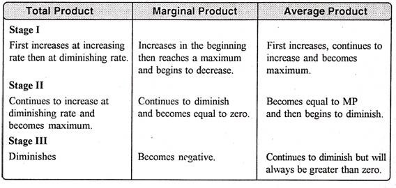
In the above table we can observe that upto the use of 3 units of labour, total product increases at an increasing rate. But after the third unit total product increases at a diminishing rate.
A marginal product is the incremental change in total product as a result of increasing the variable factor i.e., labour. We can see from the table, marginal product of labour initially rises and beyond the use of third unit it starts diminishing. The use of 6 units does not add anything in the production. Thus marginal product of labour fallen to zero. After the 6 unit, total product decreases and marginal product becomes negative.
Average product is derived by dividing total product by the quantity of variable unit. Till the 3 unit of labour, average product increases. Whereas after the 3 unit, average product is falling throughout.
Three Stages of the Law of Variable Proportions:
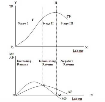
The stages are discussed in the below figure where labour is measured on the X-axis and output on the Y-axis.
Stage 1. Stage of Increasing Returns:
In this stage, total product increases at an increasing rate till point F. i.e., the curve TP concave upwards upto point F which means marginal product of labour rises. Because efficiency of fixed factor increases with the increase in variable facto labour. After point F, the total product starts increasing at a diminishing rate. Looking at the next figure, marginal product of labour is maximum, after which it diminishes. This stage is called the stage of increasing returns because the average product of the variable factor labour increases throughout this stage. This stage ends at the point where the average product curve reaches its highest point.
Stage 2. Stage of Diminishing Returns:
The stage 2 ends, when the total product increases at a diminishing rate until it reaches it maximum point H. In this stage both marginal product and average product are diminishing but remain positive. Because fixed factor land becomes inadequate with the increase in the quantity of variable factor labour. At point M marginal product is zero which corresponds to the maximum point H of the total product curve.
Stage 3. Stage of Negative Returns:
In stage 3, with the increase in variable factor labour, the total product decline. Therefore the TP curve slopes downward. As a result, marginal product of labour is negative and MP cure falls below x axis. In this case fixed factor land becomes too much inadequate to the increase in variable factor labour.
Q2) Explain returns of scale.
A2) In long run, no factors are fixed. Return of scale refers to proportionate change in productivity from proportionate change in all the inputs.
Definition:
“The term returns to scale refers to the changes in output as all factors change by the same proportion.” Koutsoyiannis.
“Returns to scale relates to the behaviour of total output as all inputs are varied and is a long run concept”. Leibhafsky.
Types of return of scale:
1. Increasing return of scale
2. Constant return of scale
3. Diminishing return of scale
Explanation
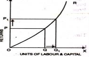
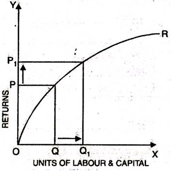
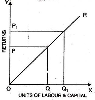
- When proportionate increase in factors of production leads to higher proportionate increase in production refers to increasing return of scale.
- In the below figure, x axis represent increase in labour and capital while Y axis represent increase in output. When labour and capital increases from Q to Q1, output also increases from P to P1 which is higher than the change in factors of production i.e., labour and capital.
2. Diminishing return of scale

3. Constant return of scale

Q3) Explain Cost Curve under Short-run and Long-run.
A3) Cost Curve under Short-run and Long-run:
Short run cost:
Short run cost is the cost where the quantity of one input is fixed and the quantity of other input varies. In this case, the land and machinery is fixed where as the other factors such as labour and capital vary with time. Thus expansion is done in hiring more labour and increasing capital.
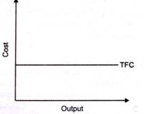
a) Total fixed cost remains fixed in short run period. The cost does not change with the change in the level of output.
b) These costs are also called indirect costs, overhead costs, historical costs, and unavoidable costs.
c) Definition
b. From the above figure , we can see TFC curve is horizontal to X axis.TFC remains constant with proportionate change in the output.
2. Total variable cost-
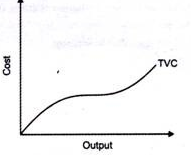
According to Ferguson, “total variable cost is the sum of amounts spent for each of the variable inputs used”
In the above figure, TVC changes with the change in the level of production
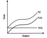
3. Total cost-
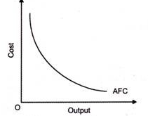
4. Average fixed cost (AFC)–
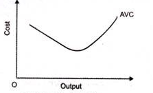
5. Average variable cost (AVC)-
c. AVC decreases as the output increases. But after a point, AVC increases as the output increases. Thus, it is U shaped curve
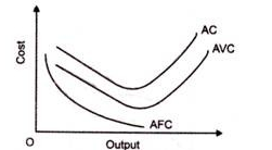
6. Average cost of production (AC)-
c. AC is also equal to the sum total of AFC and AVC. AC curve is also U-shaped curve as average cost initially decreases when output increases and then increases when output increases.
7. Marginal cost (MC)-
 Proportionate change in output
Long run cost-
In long run, all the factors of production vary. Long run is period in which all cost change as all the factors of production are variable. To produce at a lower cost in long run, the organization should have the ability to change the factors of production. There is no difference between TC and TVC as there is no fixed cost.
- It refers to the minimum cost at which a given level of output can be produced.
- Definition:
According to Leibhafasky, “the long run total cost of production is the least possible cost of producing any given level of output when all inputs are variable.”
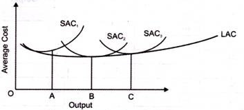
2. Long run average cost (LAC)-

3. Long run marginal cost (LMC)-

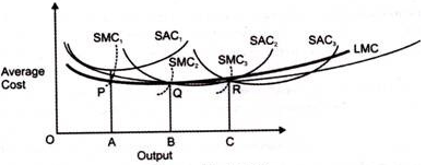
c. On the graph, Output A,B,C intersects SMC at P,Q,R. LMC is drawn by joining P,Q and R respectively which is the tangency between LAC and SAC.
Q4) Explain Relationship between Average Cost and Marginal Cost.
A4) The relationship between output and cost is expressed in terms of cost function. The companies use cost function to minimize cost and maximize production efficiently.
The following functions are applied to take decision
- It is the full cost of producing any given level of output. The cost is divided into 2 parts-
- Total fixed cost does not vary with the level of output. For ex – land
- Total variable cost changes directly with the output. For ex – labour.
2. Average cost
3. Marginal cost

Change in output
Relation between average cost and marginal cost:
Average cost can be worked out by dividing the total cost by total output.
Likewise, marginal cost can also be calculated from total cost. The addition made to the total cost by producing one more unit of the commodity is called marginal cost. MC = TCn – TCn-1
When average cost falls, marginal cost also falls. In this case, marginal cost falls more rapidly than the average cost. That is why when marginal cost curve is falling; it is below the average cost curve.
When average cost rises, marginal cost also rises but marginal cost rises more rapidly than the average cost.
MC cuts AC at its lowest point: When average cost is minimum then marginal cost will be equal to it.
For a brief stretch, AC may continue to decline even when MC is rising: Shows that between points F and E, marginal cost is rising while AC continues to fall.
Mutual Interaction between MC and AC: When marginal cost is more than average cost, average cost has a tendency to rise. It seems as if marginal cost curve is pulling the AC curve upward. On the other hand, when MC is less than AC, it pulls the AC curve downward. When MC is equal to AC then the latter is constant.
Q5) Explain Perfect Competition: Features
A5) Perfect competition refers to ‘A market structure in which there are large number of buyers and sellers with a single uniforms price for the product which is determined by the forces of demand & supply.’ The price prevailing in perfect competition market is equilibrium price.
Definition:
It is identified by the existence of the many firm; they all sell an identical products an equivalent way. The supplier is the one who accepts the price."- Vilas
Such market gains when the request for product of every producer is totally elastic. Mrs Joan Robinson.
It is a market condition with an outsized number of sellers and buyers, similar products, free entry of enterprises into the industry is ideal knowledge between buyers and sellers of existing market conditions and free mobility of production factors between alternative uses. Lim Chong-ya.
Characteristic of perfect competition:-
1) Large number of seller / seller are price takers: There are many potential sellers selling their commodity in the market. Their number is so large that a single seller cannot influence the market price because each seller sells a small fraction of total market supply. The price of the product is determined on the basis of market demand and market supply of the commodity which is accepted by the firms, thus seller is a price taker and not a price maker.
2) Large number of buyers: There are many buyers in the market. A single buyer cannot influence the price of the commodity because individual demand is a small fraction of total market demand.
3) Homogeneous product: The product sold in the market is homogeneous, i.e. identical in quality and size. There is no difference between the products. The products are perfect substitutes for each other.
4) Free entry and exit: There is freedom for new firms or sellers to enter into the market or industry. There is no legal, economic or any type of restrictions. Similarly, the seller is free to leave the market on industry.
5) Perfect knowledge: The seller and buyers have perfect knowledge about the market such as price, demand and supply. This will prevent the buyer from paying higher price than the market price. Similarly, sellers cannot change a different price than the prevailing market price.
6) Perfect mobility of factors of production: Factors of production are freely mobile from one firm to another or from one place to another. This ensures freedom of entry and exit firms. This also ensure that the factors cost are the same for all firms.
7) No transport cost: It is assumed that there are no transport costs. As a result, there is no possibility of changing a higher price on the behalf of transport costs.
8) Non intervention by the government: It is assumed that government does not interfere in the working of the market economy. Price is determined freely according to demand and supply conditions of the market.
9) Single Price: In Perfect Competition all units of a commodity have uniforms or a single price. It is determined by the forces of demand and supply.
Q6) Explain prefect competition Equilibrium of Firm/ industry.
A6) Equilibrium of firm and industry:
Equilibrium refers to when the firm has no inclination to expand or to contract its output. The producer can attain equilibrium under two situations.
The Marginal Revenue-Marginal Cost Approach
Profit depends on revenue and cost. Thus equilibrium revolves around revenue and cost. According to the MR-MC approach, a producer is said to be in equilibrium when:
- A Firm can maximise the profit when marginal revenue is equal to marginal cost
- MR is the addition to TR from the sale of one more unit.
- MC is the addition to TC when an additional unit is produced.
- Thus when MR = MC, TR-TC result in maximum profit.
- If MR exceeds MC, then producer will produce more as it adds to the profit.
- MC= MR is a necessary condition, but its is not enough to ensure equilibrium. This condition happens more than one output level.
- To ensure equilibrium, it has to be supplemented by the condition that MR should be less than MC after this level.
Producer’s Equilibrium when Price remains Constant
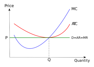
Price remains constant under conditions of perfect competition. Here price is equal to AR. When price is constant, revenue from each additional unit is equal to AR. It means AR curve is same as MR curve. The firm attains equilibrium when two condition are fulfilled , that is firm aims at producing that level of output at which MC is equal to MR and MC is greater than MR after MC = MR output level.
Producer’s Equilibrium when Price is not Constant

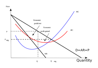
When there is no fixed price, price falls with an increase in output. The producer sells more units at a lower price. In this case MR slopes downwards. The firm aims at producing that level of output at which MC is equal to MR and MC is greater than MR.
Short run and long run supply curves-
Supply curve shows the relationship between price and quantity supplied. According to Dorfman, “Supply curve is that curve which indicates various quantities supplied by the firm at different prices”.
Supply curve can be divided into two parts as:
Short run supply curve of a firm
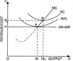
Under Short run , fixed cost remains constant, supply can be changed by changing the only the variable factors. Thus the firm has to bear fixed cost id it is shut down. Thus in short run, goods are supplied at price is either greater or equal to average variable cost. Average revenue is equal to marginal revenue under perfect competition. Hence the firm will produce at the point where marginal revenue and marginal cost are equal.
Prof. Bilas has defined it in simple words, “The Firm’s short period supply curve is that portion of its marginal cost curve that lies-above the minimum point of the average variable cost curve.”
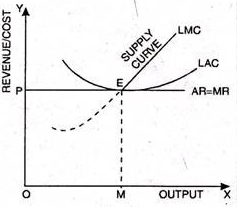
From the above figure we can see that, the firm will not be covering its average variable cost, at price less than OP. At price OP, OM is the supply. MC and MR cut at point A, OM is equilibrium output. If price rise to OP1, the firm will produce OM1 output. This short run supply curve of a firm starts from A upwards i.e., thick line AB.
Long run supply curve
Under long run, the supply curve changes by changing all the factors of production. The firm produces only at minimum average cost in long run. In this case, long run marginal cost, marginal revenue, average revenue and long run average cost are equal. The firm enjoys normal profit.
Optimum production is the point where minimum average cost is equal to marginal cost. Long run supply curve is a portion where marginal cost curve that lies above the minimum point of the average cost curve.
Optimum point is the Point E, as at this point MR=LMCAR minimum LAC. The portion of LMC above point E is called long run supply curve
Q7) Explain Role of Time element in Price Determination.
A7) Role of Time element in Price Determination-
According to Marshall ,time has great influence on the determination of price .The following are the market periods based on time- market period, short period and long period.
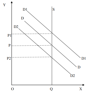
Market period or very short period may be only a day or very few days .Change in supply is not possible where the period is very short and quantity demanded will be the determining factor in this period Further, supply curve in the market period is remain fixed showing vertical straight line. The short period is a period not sufficient to make any changes in the existing fixed plant capacity. Increase in supply in the short period is possible by increasing the variable factors of production only The supply curve slopes upward to right showing that some increase in supply is possible when the price increases.
Long period is a time long enough to adjust the supply to any changes in demand. The long run supply curve is less steep then short run supply curve showing increase in quantity supplied when price changes.
During the Market period
In very short period ,supply is inelastic ,thus the price depends on changes in demand .The supply curve will be vertical straight line parallel to y-axis.
In the above diagram, SP is the supply curve. It means where ever the price is ,the fixed supply is to be sold in the market .Here DD is the demand curve .The supply is SQ .The point of equilibrium is at „S‟ so the equilibrium is OP. Here the demand alone determines the price because supply is fixed. If the demand increases to D1D1, the price will increase from OP to OP1 and vice versa ,ie, if the demand decreases to D2D2 , the price will decrease to OP2.
If the commodity is non- perishable, It can be stored .The seller does not sell the goods if the price is low. But the price is high he will sell whole stock .The curve will be curved at beginning ;then it will become a straight line .Under very short period , the demand alone determines the price.
During short period
In this period ,the firm can make slight changes in their supply of goods without changing the capacity of plant.
In this diagram ,DD is the demand curve and SS is the supply curve. At point „E‟ the demand curve equals the supply curve ,the equilibrium price is OP.If the demand is increased to D1D1 the equilibrium price will be OP1 and if the demand decreased to D2D2 , the equilibrium will be OP2. But the quantity will be decreased from OQ to OQ2. The firm in the short run can produce output by increasing the variable inputs. . A firm gets maximum profit where MC=MR .The price determination by the industry is given in the following diagram.
In the above diagram, it can be revealed that the price is determined by the industry OP. when the demand is shifted to D1D1 then the quantity demanded is decreased from OQ to OQ1 and also price decreases from OP to OP1. In the case of a firm, MR=AR, thus demand =AR=MR=price
In the long run
In the long run , the firms in the industry are eager to get super normal profits . The price determination is explained through the diagram given below; In output decision making in the long run .Long run Average Cost (LAC) and Long run Marginal Cost (LMC) are to be taken in to consideration . under this condition ,the firm is in equilibrium
When AR=MR=LAC=LMC

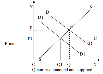
In the above diagram. (1) DD is the long run . Demand curve and S1 S1 short run supply curve .The price is determined at OP.In the figure 2,the equilibrium output is at point E. At this point .AR1=MR=LMC
Q8) Explain Monopoly: Feature, Equilibrium of Firm/Industry.
A8) The word monopoly has been derived from the combination of two words i.e., ‘Mono’ and ‘Poly’. Mono refers to a single and poly to control.
Thus, monopoly refers to a market situation in which there is only one seller of a commodity.
In monopoly market, single firm or one seller controls the entire market. The firm has all the market power, so he can set the prices to earn more profit as the consumers do not have any alternative.
Definition
“Pure monopoly is represented by a market situation in which there is a single seller of a product for which there are no substitutes; this single seller is unaffected by and does not affect the prices and outputs of other products sold in the economy.” Bilas
“Monopoly is a market situation in which there is a single seller. There are no close substitutes of the commodity it produces, there are barriers to entry”. –Koutsoyiannis
“A pure monopoly exists when there is only one producer in the market. There are no dire competitions.” –Ferguson
Features-
2. No Close Substitutes - There is no close substitutes for the product sold by the monopolist. The cross elasticity of demand between the product of the monopolist and others must be negligible or zero.
3. Difficulty of Entry of New Firms - There are restrictions on the entry of firms into the industry, even when the firm is making abnormal profits. Other sellers are unable to enter the market of the monopoly
4. Profit maximize - A monopoly maximizes profits. Due to the lack of competition a firm can charge a set price above what would be charged in a competitive market, thereby maximizing its revenue.
5. Price Maker - Under monopoly, monopolist has full control over the supply of the commodity. The price is set by determining the quantity in order to demand the price desired by the firm. Therefore, buyers have to pay the price fixed by the monopolist.
Equilibrium
A. Short run
A monopolist maximizes his short-term profits if the following two conditions are met first, MC equals Mr. Secondly; the slope of MC is larger than that of Mr at the intersection.
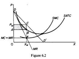
In Figure 6.2, the equilibrium of the monopoly is defined by the point θ at which MC intersects the MR curve from below. Thus, both conditions of equilibrium are met. The price is PM and the quantity is XM. Monopolies realize excess profits equal to shaded areas APM CB. Please note that the price is higher than Mr
In pure competition, the company is the one who receives the price, so it’s only decision is the output decision. The monopolist is faced with two decisions: to set his price and his output. But given the downward trend demand curve, the two decisions are interdependent.
Monopolies set their own prices and sell the amount the market takes on it, or produce an output defined by the intersection of MC and MR and are sold at the corresponding price. An important condition for maximizing the profits of monopolies is the equality of the MC and the MR, provided that the MC cuts the MR from below.
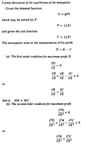

We can now revisit the statement that there is no unique supply curve for the monopolist derived from his MC. Given his MC, the same amount could be offered at different prices depending on the price elasticity of demand. This is graphically shown in Figure 6.3. Quantity X is sold at price P1 if demand is D1, and the same quantity X is sold at price P2 if demand is D2.
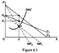
So there is no inherent relationship between price and quantity. Similarly, given the monopolist MC, we can supply various quantities at any one price, depending on the market demand and the corresponding MR curve. Figure 6.4 illustrates this situation. The cost condition is represented by the MC curve. Given the cost of a monopolist, he would supply 0X1 if the market demand is D1, then p at the same price, and only 0X2 if the market demand is D2 B.Long-term equilibrium:
In the long run the monopolist will have time to expand his plants or use his existing plants at every level to maximize his profits. However, if the entry is blocked, the monopolist does not need to reach the optimal scale (that is, the need to build the plant until the minimum point of LAC is reached), neither does the guarantee that he will use his existing plant at the optimum capacity. What is certain is that if he makes a loss in the long run, the monopolist will not stay in business.
He will probably continue to earn paranormal benefits even in the long run, given that entry is banned. But the size of his plant and the degree of utilization of any plant size depends entirely on the market demand. He may reach the optimal scale (the minimum point of Lac), stay on the less optimal scale (the falling part of his LAC), or exceed the optimal scale (expand beyond the minimum LAC), depending on market conditions.
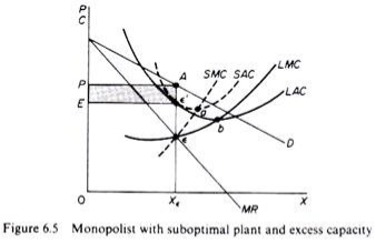
Figure 6.5 shows when the market size does not allow the monopolist to expand to the minimum point of Lac. In this case, not only is his plant not optimal (in the sense that the economy of full size is not depleted), but also the existing plant is not fully utilized. This is because on the left of the minimum point of the LAC, the SRAC touches the LAC at its falling part, and the short-term MC must be equal to the LRMC. This happens in e, but the minimum LAC is b,and the optimal use of the existing plant is a. Since it is utilized at Level E', there is excess capacity. Finally, figure 6.7 shows a case where the market size is large enough for a monopolist to build an optimal plant and be able to use it at full capacity.
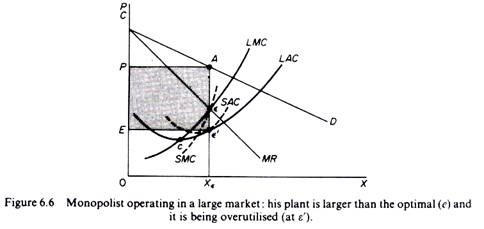
In Figure 6.6, the scale of the market is so large that monopolists have to build plants larger than the optimal ones to maximize output and over-exploit them. This is because to the right of the minimum point of LAC, SRAC and LAC is tangent at the point of positive slope, and SRMC must be equal to LAC. Thus, plants that maximize the profits of monopolies are, firstly, larger than the optimal size, and secondly, they are over-utilized, which leads to higher costs. This is often the case with utility companies operating at the state level.
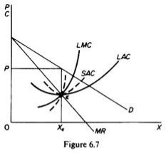
It should be clear that which of the above situations will appear in a particular case will depend on the size of the market (given the technology of monopolists). There is no certainty that monopolies will reach their optimal size in the long run, as is the case with purely competitive markets. In Monopoly, there is no market force similar to those of pure competition that will lead companies to operate at optimal plant size in the long run (and utilize it at its full capacity).
Q9) Explain Monopolistic Combination: Features, Price-Output Policy of the Firm.
A9) Monopolistic competition:
In Monopolistic competition there are large numbers of buyers and sellers which do not sell homogenous product unlike perfect competition. This is more realistic in the real world. Monopolistic competition occurs when an industry in which many firms selling products that are similar but not identical.
Monopolistic competitions try to differentiate its product. Thus it is closely related to business strategy of brand differentiation. In monopolistic competition heavy advertising and marketing is common among firms.
Monopolistic competition combines element of both monopoly and perfect competition. All firms in monopolistic competition relatively have low market power and they are all market makers.
Monopolistic competitive market -
Features
2. Many firms – there are many firms in each product group. A product group is a "collection of similar products". Under monopolistic market, each firms has a small market share. This gives each firm a freedom to set price and each firm action have negligible impact on the market. A firm can cut the price to increase sale without any fear. As its action will not prompt retaliatory responses from competitors.
3. Freedom of entry and exit - Like perfect competition, under monopolistic competition the firms can freely enter or exit. When the existing firms makes super-normal profits, then new firms will enter. The entry of new firms leads to increase the supply of goods and services and this would reduce the price and thus the existing firms will be left only with normal profits. Similarly, if the existing firms are incurring losses, some of the firms will exit. This will reduce the supply which result decrease in price and the existing firms will be left only with normal profit.
4. Independent decision making – under monopolistic market, each firm can independently sets the terms and conditions of exchange for its product. The firm does not consider how their decision will have impact on competitors. In other words, each firm feels free to set prices and prompting heightened competition.
5. Market power – under monopolistic competition, the firms have low degree of market power. Market power means that the firm has control over the terms and conditions of exchange for its product. All firms under monopolistic competition are price makers. A firm can raise the prices of products and services without losing all its customers base. The firm can also lower prices without any effect on the competitors. Since the firm have relatively low market power, there is no barrier to entry.
Monopolistic competition price and output decision-equilibrium
Under monopolistic competition a firm can some extent independently control the supply and price of the product. The demand curve is stable and slightly downward slope
A monopolistic competitor creates output at which the marginal cost is equal to marginal revenue. The price is greater than marginal cost.
Short run-
In short run, the firm attains its equilibrium where marginal revenue equals marginal cost and the price is set according to its demand curve. Thus when MR=MC, profits are maximized

In the above fig,
AR is the average revenue curve,
MR represents the marginal revenue curve,
SAC curve represents the short run average cost curve,
SMC signifies the short run marginal cost.
In the above figure we can see that at output OM, MR intersects SMC. Here price is OP’ (which is equal to MP). Thus P is the point on AR curve, which is price. PT is the supper normal profit per unit output, is the difference between the average revenue and average cost.
Long run-
In the long run due to the possibility of new firms entering the industry the price under monopolistic competition becomes equal to long-run average cost giving only normal profits. So, no firm under monopolistic competition can make excess profit or loss in the long run.
When the new firm start supplying, the price would fall. Thus the AR curve shifts from right to left and supernormal profits are replaced with normal profits. The long run equilibrium is achieved when average revenue is equal to average cost.

In the above fig we can see that, at point P, AR curve touches the average cost curve (LAC) as a tangent. P is the equilibrium at price MP and output OM.
At MP average cost is equal to average revenue. Therefore, in long run, the profit is normal. The conditions (MR=MC and AR=AC) result in attaining equilibrium in long run.
Q10) Explain Selling Cost, Meaning, Effects, Equilibrium of Firm with respect to Selling Cost.
A10) Unlike a perfectly competitive firm, in order to increase the sale of the product the monopolist has to undertake huge advertising campaigns. In perfect competitions, product manufactured by different firms are homogenous, there must be uniformity of price. But in case of monopolistic competition, product differentiation is the common feature and for this reason selling cost would be crucial.
According to Chamberlin, “Selling costs are those costs which are to be incured in order 10 alter the position or shape of the demand curve for a product.” In words of Cairn cross, “Selling costsinc1ude all expenditure designed to create, increase or maintain me demand for a firms output.
Effect of Selling Costs on Price Determination under Monopolistic Competition:
Under monopolistic competition, selling costs increase demand for the product as well as the cost of production. The main objectives the firm is to maximise the profit. When the firm incurs an expenditure on selling costs, there will be shift of its demand and cost curves. The firm will continue to incur expenditure on advertisement, so long as, revenue earned is more than or equal to cost of advertisement. The equilibrium of the firm under the selling cost has been explained below.
Assumption:
Average selling cost-
The curve of selling cost is a tool of economic analysis. It is a curve of average selling cost per unit of product. It is akin to the average cost curves. In other words, like the cost curves, selling costs are also of U-shape. Moreover, there are two terms according to which the curve of selling cost is drawn. But, in both the cases, the shape of selling cost differs from one another.

In the initial stage, the curve falls and later it starts rising. It means in the beginning proportionate increase in sale is more than the increase in selling costs, but after a point proportionate increase in sale is less than the selling cost. It signifies the fact that up to a certain level per unit selling cost go on to diminish but after that the same tend to increase. But, the ASC neither will touch the X-axis nor it will be zero. In other words, the ASC will form the shape of rectangular hyperbola.
Equilibrium with Selling Costs (Variable Costs):
Selling costs influence equilibrium price-output adjustment of a firm under monopolistic competition. In the Fig. below. APC is the initial average production cost. AR1 is the initial average revenue curve or initial demand curve. The initial price is OP and the firm earns profits shown by the first shaded rectangle PQRS.
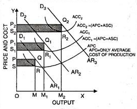
ACC1 is the average composite costs curve, which includes the average selling cost (ASC). Average selling cost is equal to the vertical distance between APC and ACQ. The new demand curve is AR2. It is obtained after incurring selling costs or after making advertisements.
It is, obvious, that the demand for the product has increased as a result of selling costs. The profits have also increased as a result of selling costs. The profits after incurring selling costs at OM1 level of output become equal to the shaded area P1Q1R1S1. Now these profits are greater than the initial level of profits when no selling cost is incurred, i.e., P1 Q1 R1 S1 > PQRS.
ACC2 is the average composite cost when more additional cost is incurred, as a result of which the demand for the product further increases. The new demand curve is AR3 which indicates a higher demand for the product. The profits are also greater than before since the shaded area P2Q2R2S2 > P1Q1R1S.
It is, thus, obvious that the demand for the product is increasing as a result of the selling costs. Since selling costs are included in the cost of production, therefore price of the product is also increasing as a result of selling costs. Profits are also increasing as a result of higher selling costs and increased demand. In the above diagram, the effect of selling outlay on competitive advertisement has been indicated. Before selling costs are incurred, the firm’s average revenue or demand curve is AR1 and APC is the basic initial cost of production.
So, the firm earns maximum profits as shown by the shaded area PQRS. Here, question arises, how long a firm may go on incurring expenditure on selling costs? It will continue to make expenditure on selling costs as long as any addition to the revenue is greater than the addition to the selling costs. The firm will stop incurring expenditure on selling costs when the total profits are at the highest possible level.
This would be the point at which the additional revenue due to advertising expenditure equals the extra expenditure on advertisement. It should, however, be noted clearly that the effects of advertisement on prices and output are uncertain. Advertisement by a firm may be considered successful if the elasticity of demand for its product falls.
Equilibrium with Selling Costs (Fixed Costs):
In modern times, a lot of money is spent on selling costs. Of course, it becomes difficult to determine the most profitable output. At the same time, we also know that selling costs create a new demand curve. However, here equilibrium is determined when there are fixed selling costs as shown in Figure below

AR is the average revenue or demand curve. MR is the marginal revenue curve. The average production cost (APC), the shaded area B shows the selling cost. This shows that by adding selling cost in average production cost, we get average total cost. (ATUC = APC + SC) SC is the net return per unit while SQ is the price minus SC – the average total unit cost and OQ is the level of output. Thus shaded area PRCS is the maximum net return and OQSP is the total revenue minus total cost OQCR.