Unit 4
Measures of Dispersion
Question and Answer
Q1) explain moments
Solution
Moments
Moments are a set of statistical parameters to measure a distribution. Four moments are commonly used:
• 1st moment - Mean (describes central value)
• 2nd moment - Variance (describes dispersion)
• 3rd moment - Skewness (describes asymmetry)
• 4th moment - Kurtosis (describes peakedness)
The formula for calculating moments is as follows:
1st moment = 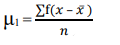
2nd moment =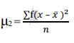
3rd moment = 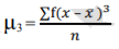
4th moment =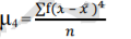
Raw Moments and Central Moments
The n-th moment about zero of a probability density function f(x) is the expected value of Xn and is called a raw moment or crude moment. The moments about its mean μ are called central moments; these describe the shape of the function, independently of translation.
A moment  of a probability function
  taken about 0,
 |  |  | (1) |
 |  |  | (2) |
The raw moments  (sometimes also called "crude moments") can be expressed as terms of the central moments
  (i.e., those taken about the mean
  ) using the inverse binomial transform
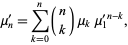 | (3) |
With  and
and  (Papoulis 1984, p. 146). The first few values are therefore
 |  |  | (4) |
 |  |  | (5) |
 |  |  | (6) |
 |  |  | (7) |
The raw moments  can also be expressed in terms of the cumulates
  by exponentiating both sides of the series
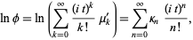 | (8) |
Where  is the characteristic function, to obtain
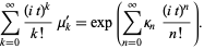 | (9) |
The first few terms are then given by
 |  |  | (10) |
 |  |  | (11) |
 |  |  | (12) |
 |  |  | (13) |
 |  |  | (14) |
The raw moment of a multivariate probability function  can be similarly defined as
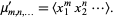 | (15) |
Therefore,
 | (16) |
The multivariate raw moments can be expressed in terms of the multivariate cumulants. For example,
 |  |  | (17) |
 |  |  | (18) |
In probability theory and statistics, a central moment is a moment of a probability distribution of a random variable about the random variable's mean; that is, it is the expected value of a specified integer power of the deviation of the random variable from the mean. The various moments form one set of values by which the properties of a probability distribution can be usefully characterized. Central moments are used in preference to ordinary moments, computed in terms of deviations from the mean instead of from zero, because the higher-order central moments relate only to the spread and shape of the distribution, rather than also to its location.
Sets of central moments can be defined for both univariate and multivariate distributions.
Q2) Calculate Bowley’s Coefficient of Skewness from the following test scores:
Sl. N o | Test scores |
1 | 17 |
2 | 17 |
3 | 26 |
4 | 27 |
5 | 30 |
6 | 30 |
7 | 31 |
8 | 37 |
Solution:
First quartile (Q1)
Qi= [i * (n + 1) /4] th observation
Q1= [1 * (8 + 1) /4] th observation
Q1 = 2.25 th observation
Thus, 2.25 th observation lies between the 2nd and 3rd value in the ordered group, between frequency 17 and 26
First quartile (Q1) is calculated as
Q1 = 2nd observation +0.75 * (3rd observation - 2nd observation)
Q1 = 17 + 0.75 * (26 – 17) = 23.75
Second quartile( )
)
Q2= [2 * (8 + 1) /4] th observation
Q2 = 4.5th Observation
So, 4.5th observation lies between 4th and 5th value in ordered group, between frequency 27 and 30.
Hence Q2 = 4th observation + 0.50 * (5th observation – 6th observation)
Q2 = 27 + 0.50 * (30 – 27) = 28.5
Third quartile (Q3)
Qi= [i * (n + 1) /4] th observation
Q3= [3 * (8 + 1) /4] th observation
Q3 = 6.75 th observation
So, 6.75 th observation lies between the 6th and 7th value in the ordered group, between frequency 30 and 31
Third quartile (Q3) is calculated as
Q3 = 6th observation +0.25 * (7th observation – 6th observation)
Q3 = 30 + 0.25 * (31 – 30) = 30.25
Therefore, Bowley’s Coefficient of Skewness is calculated as under:
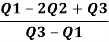
= 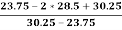
=  = - 0.461
Q3) Below are the data of hours spent watching television by the 220 students. Calculate Karl Pearsons Co-efficient of Skewness.
Hours | No. Of students |
10 – 14 | 2 |
15 – 19 | 12 |
20 – 24 | 23 |
25 – 29 | 60 |
30 – 34 | 77 |
35 – 39 | 38 |
40 - 44 | 8 |
Solution:
Hours | No. Of students | x | Fx |  |  |  |
10 – 14 | 2 | 12 | 24 | -17.82 | 317.49 | 634.98 |
15 – 19 | 12 | 17 | 204 | -12.82 | 164.31 | 1971.67 |
20 – 24 | 23 | 22 | 506 | -7.82 | 61.12 | 1405.85 |
25 – 29 | 60 | 27 | 1620 | -2.82 | 7.94 | 476.53 |
30 – 34 | 77 | 32 | 2464 | 2.18 | 4.76 | 366.55 |
35 – 39 | 38 | 37 | 1406 | 7.18 | 51.58 | 1959.98 |
40 - 44 | 8 | 42 | 336 | 12.18 | 148.40 | 1187.17 |
| 220 |
| 6560 |
|
| 8002.73 |

Mean = 6560/220 = 29.82

SD = √8002.73/220 = 6.03
 Mode = L1 + (L2 – L1) d1
d1 +d2
Here modal class is 30 – 34 (Since the frequency is highest)
L1 = 30, L2 = 34, d1 = 17, d2 = 39
 Mode = 30 + (34 – 30) 17
17 + 39
Mode = 30 +  x 17
x 17
= 30 + 1.21
= 31.21
Therefore, Co-efficient of Skewness
 =
= 
= 
= - 0.23
Q4) the frequency table shows the number of goals the lakers scored in their last twenty matches. What was the range
No. Of goals | Frequency |
0 | 2 |
1 | 3 |
2 | 3 |
3 | 6 |
4 | 3 |
5 | 1 |
6 | 1 |
7 | 1 |
Solution
The range is the difference between the lowest and highest values.
The highest value was 7 (They scored 7 goals on 1 occasion)
The lowest value was 0 (They scored 0 goals on 2 occasions)
Therefore the range = 7 - 0 = 7
Q5) calculate quartile deviation from the following test scores
Sl. N o | Test scores |
1 | 17 |
2 | 17 |
3 | 26 |
4 | 27 |
5 | 30 |
6 | 30 |
7 | 31 |
8 | 37 |
Solution
First quartile (Q1)
Qi= [i * (n + 1) /4] th observation
Q1= [1 * (8 + 1) /4] th observation
Q1 = 2.25 th observation
Thus, 2.25 th observation lies between the 2nd and 3rd value in the ordered group, between frequency 17 and 26
First quartile (Q1) is calculated as
Q1 = 2nd observation +0.75 * (3rd observation - 2nd observation)
Q1 = 17 + 0.75 * (26 – 17) = 23.75
Third quartile (Q3)
Qi= [i * (n + 1) /4] th observation
Q3= [3 * (8 + 1) /4] th observation
Q3 = 6.75 th observation
So, 6.75 th observation lies between the 6th and 7th value in the ordered group, between frequency 30 and 31
Third quartile (Q3) is calculated as
Q3 = 6th observation +0.25 * (7th observation – 6th observation)
Q3 = 30 + 0.25 * (31 – 30) = 30.25
Now using the quartiles values Q1 and Q3, we will calculate the quartile deviation.
QD = (Q3 - Q1) / 2
QD = (30.25 – 23.75) / 2 = 3.25
Q6) computation of quartile deviation for grouped test scores
Class | Frequency |
9.3-9.7 | 22 |
9.8-10.2 | 55 |
10.3-10.7 | 12 |
10.8-11.2 | 17 |
11.3-11.7 | 14 |
11.8-12.2 | 66 |
12.3-12.7 | 33 |
12.8-13.2 | 11 |
Solution
Class | Frequency | Class boundaries | CF |
9.3-9.7 | 2 | 9.25-9.75 | 2 |
9.8-10.2 | 5 | 9.75-10.25 | 2 + 5 = 7 |
10.3-10.7 | 12 | 10.25-10.75 | 7 + 12 = 19 |
10.8-11.2 | 17 | 10.75-11.25 | 19 + 17 = 36 |
11.3-11.7 | 14 | 11.25-11.75 | 36 + 14 = 50 |
11.8-12.2 | 6 | 11.75-12.25 | 50 + 6 = 56 |
12.3-12.7 | 3 | 12.25-12.75 | 56 + 3 = 59 |
12.8-13.2 | 1 | 12.75-13.25 | 59 + 1 = 60 |
First quartile (Q1)
Qi= [i * (n ) /4] th observation
Q1 = [1*(60)/4]th observation
Q1 = 15th observation
So, 15th value is in the interval 10.25-10.75
Group of Q1 = 10.25-10.75
Qi = (I + (h / f) * ( i * (N/4) – c) ; i = 1,2,3
Q1 = (10.25 + ( 0.5/ 12)* (1* (60/4) – 7)
Q1 = 10.58
Third quartile (Q3)
Qi= [i * (n) /4] th observation
Q3= [3 * (60) /4] th observation
Q3 = 45th observation
So, 45th value is in the interval 11.25-11.75
Group of Q3 = 11.25-11.75
Qi = (I + (h / f) * ( i * (N/4) – c) ; i = 1,2,3
Q3 = (11.25 + ( 0.5/ 14)* (3* (60/4) – 36)
Q3 = 11.57
QD = (Q3 - Q1) / 2
QD = (11.57 – 10.58) / 2 = 0.495
Q7) Computation of Mean deviation in grouped data
Class interval | 15 – 19 | 20 – 24 | 25 – 29 | 30 – 34 | 35 – 39 | 40 – 44 | 45 - 49 |
Frequency | 1 | 4 | 6 | 9 | 5 | 3 | 2 |
Solution
Class Interval | F | X | FX | D | FD |
15 – 19 | 1 | 17 | 17 | 15 | 15 |
20 – 24 | 4 | 22 | 88 | 10 | 40 |
25 – 29 | 6 | 27 | 162 | 5 | 30 |
30 - 34 | 9 | 32 | 288 | 0 | 0 |
35 - 39 | 5 | 37 | 185 | 5 | 25 |
40 - 44 | 3 | 42 | 126 | 10 | 30 |
45 - 49 | 2 | 47 | 94 | 15 | 30 |
| N = 30 |
| ∑fx = 960 |
|  |
Mean = 960/30 = 32
MD = 170 / 30 = 5.667
Coefficient of mean deviation
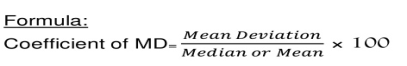
Coefficient of mean deviation = (5.67/32)*100 = 17.71
Q8) calculate mean deviation from the median
Class | 5 -15 | 15 - 25 | 25 - 35 | 35 - 45 | 45 – 55 |
Frequency | 5 | 9 | 7 | 3 | 8 |
Solution
x | f | Cf | Midpoint x | x –median | F(x-m) |
5 -15 | 5 | 5 | 10 | 17.42 | 87.1 |
15 -25 | 9 | 14 | 20 | 7.42 | 66.78 |
25 -35 | 7 | 21 | 30 | 2.58 | 18.06 |
35 -45 | 3 | 24 | 40 | 12.58 | 37.74 |
45- 55 | 8 | 32 | 50 | 22.58 | 180.64 |
| 32 |
|
|
| 390.32 |
Since n/2 = 32/2 = 16, therefore the class is 25 – 35 is the median.
Median = 
 Median = 25+16-14 *10 = 27.42
7
MD from median is 390.32/32 = 12.91
Q9) calculate the standard deviation using the direct method
Class interval | Frequency |
30 – 39 | 3 |
40 – 49 | 1 |
50 – 59 | 8 |
60 – 69 | 10 |
70 – 79 | 7 |
80 – 89 | 7 |
90 – 99 | 4 |
Solution
Class interval | Frequency | Midpoint x | Fx |  |  |  |
30 – 39 | 3 | 34.5 | 103.5 | -33.5 | 1122.25 | 3366.75 |
40 – 49 | 1 | 44.5 | 44.5 | -23.5 | 552.25 | 552.25 |
50 – 59 | 8 | 54.5 | 436.0 | -13.5 | 182.25 | 1458 |
60 – 69 | 10 | 64.5 | 645.0 | -3.5 | 12.25 | 122.5 |
70 – 79 | 7 | 74.5 | 521.5 | 6.5 | 42.25 | 295.75 |
80 – 89 | 7 | 84.5 | 591.5 | 16.5 | 272.25 | 1905.75 |
90 – 99 | 4 | 94.5 | 378.0 | 26.5 | 702.25 | 2809 |
| 40 |
| 2720 |
|
| 10510 |

Mean = 2720/40 = 68

SD = √10510/40 = 16.20
.
Q10) calculate the mean and standard deviation of hours spent watching television by the 220 students.
Hours | No. Of students |
10 – 14 | 2 |
15 – 19 | 12 |
20 – 24 | 23 |
25 – 29 | 60 |
30 – 34 | 77 |
35 – 39 | 38 |
40 - 44 | 8 |
Solution
Hours | No. Of students | x | Fx |  |  |  |
10 – 14 | 2 | 12 | 24 | -17.82 | 317.49 | 634.98 |
15 – 19 | 12 | 17 | 204 | -12.82 | 164.31 | 1971.67 |
20 – 24 | 23 | 22 | 506 | -7.82 | 61.12 | 1405.85 |
25 – 29 | 60 | 27 | 1620 | -2.82 | 7.94 | 476.53 |
30 – 34 | 77 | 32 | 2464 | 2.18 | 4.76 | 366.55 |
35 – 39 | 38 | 37 | 1406 | 7.18 | 51.58 | 1959.98 |
40 - 44 | 8 | 42 | 336 | 12.18 | 148.40 | 1187.17 |
| 220 |
| 6560 |
|
| 8002.73 |

Mean = 6560/220 = 29.82

SD = √8002.73/220 = 6.03


