Unit - 2

Relational Data Model

Q1) Explain in brief relational data model?

A1) Relational data model is the primary data model, which is used widely around the world for data storage and processing. This model is simple and it has all the properties and capabilities required to process data with storage efficiency.

Concepts

Tables−In relational data model, relations are saved in the format of Tables. This format stores the relation among entities. A table has rows and columns, where rows represents records and columns represent the attributes.

Tuple− A single row of a table, which contains a single record for that relation is called a tuple.

Relation instance− A finite set of tuples in the relational database system represents relation instance. Relation instances do not have duplicate tuples.

Relation schema− A relation schema describes the relation name (table name), attributes, and their names.

Relation key−Each row has one or more attributes, known as relation key, which can identify the row in the relation (table) uniquely.

Attribute domain−Every attribute has some predefined value scope, known as attribute domain.

Constraints

Every relation has some conditions that must hold for it to be a valid relation. These conditions are called Relational Integrity Constraints. There are three main integrity constraints −

●        Key constraints

●        Domain constraints

●        Referential integrity constraints

Key Constraints

There must be at least one minimal subset of attributes in the relation, which can identify a tuple uniquely. This minimal subset of attributes is called key for that relation. If there are more than one such minimal subsets, these are called candidate keys.

Key constraints force that −

• In a relation with a key attribute, no two tuples can have identical values for key attributes.
• A key attribute cannot have NULL values
• Key constraints are also referred to as Entity Constraints.

Domain Constraints

Attributes have specific values in real-world scenario. For example, age can only be a positive integer. The same constraints have been tried to employ on the attributes of a relation. Every attribute is bound to have a specific range of values. For example, age cannot be less than zero and telephone numbers cannot contain a digit outside 0-9.

Referential integrity Constraints

Referential integrity constraints work on the concept of Foreign Keys. A foreign key is a key attribute of a relation that can be referred in other relation.

Referential integrity constraint states that if a relation refers to a key attribute of a different or same relation, then that key element must exist.

Q2) Write short notes on database schema and database instance?

A2) Database Schema

A database schema is the skeleton structure that represents the logical view of the entire database. It defines how the data is organized and how the relations among them are associated. It formulates all the constraints that are to be applied on the data.

A database schema defines its entities and the relationship among them. It contains a descriptive detail of the database, which can be depicted by means of schema diagrams. It’s the database designers who design the schema to help programmers understand the database and make it useful.

Fig 1 - Database schema

A database schema can be divided broadly into two categories −

●        Physical Database Schema−This schema pertains to the actual storage of data and its form of storage like files, indices, etc. It defines how the data will be stored in a secondary storage.

●        Logical Database Schema−This schema defines all the logical constraints that need to be applied on the data stored. It defines tables, views, and integrity constraints.

Database Instance

It is important that we distinguish these two terms individually. Database schema is the skeleton of database. It is designed when the database doesn't exist at all. Once the database is operational, it is very difficult to make any changes to it. A database schema does not contain any data or information.

A database instance is a state of operational database with data at any given time. It contains a snapshot of the database. Database instances tend to change with time. A DBMS ensures that its every instance (state) is in a valid state, by diligently following all the validations, constraints, and conditions that the database designers have imposed.

Q3) Explain in brief integrity constraints?

A3) Integrity Constraints

●        Integrity constraints are a set of rules. It is used to maintain the quality of information.

●        Integrity constraints ensure that the data insertion, updating, and other processes have to be performed in such a way that data integrity is not affected.

●        Thus, integrity constraint is used to guard against accidental damage to the database.

Types of Integrity Constraint

Fig 2 - Integrity Constraint

1. Domain constraints

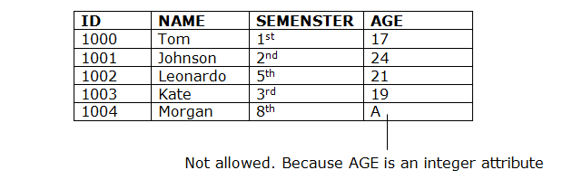
●        Domain constraints can be defined as the definition of a valid set of values for an attribute.

●        The data type of domain includes string, character, integer, time, date, currency, etc. The value of the attribute must be available in the corresponding domain.

Example:

2. Entity integrity constraints

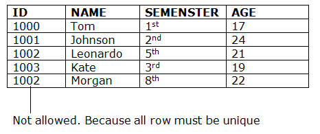
●        The entity integrity constraint states that primary key value can't be null.

●        This is because the primary key value is used to identify individual rows in relation and if the primary key has a null value, then we can't identify those rows.

●        A table can contain a null value other than the primary key field.

Example:

3. Referential Integrity Constraints

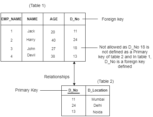
●        A referential integrity constraint is specified between two tables.

●        In the Referential integrity constraints, if a foreign key in Table 1 refers to the Primary Key of Table 2, then every value of the Foreign Key in Table 1 must be null or be available in Table 2.

Example:

4. Key constraints

●        Keys are the entity set that is used to identify an entity within its entity set uniquely.

●        An entity set can have multiple keys, but out of which one key will be the primary key. A primary key can contain a unique and null value in the relational table.

Example:

Q4) What is Foreign Key in DBMS?

A4) Foreign key

A foreign key is different from a super key, candidate key or primary key because a foreign key is the one that is used to link two tables together or create connectivity between the two.

Here, in this section, we will discuss foreign key, its use and look at some examples that will help us to understand the working and use of the foreign key. We will also see its practical implementation on a database, i.e., creating and deleting a foreign key on a table.

What is a Foreign Key

A foreign key is the one that is used to link two tables together via the primary key. It means the columns of one table points to the primary key attribute of the other table. It further means that if any attribute is set as a primary key attribute will work in another table as a foreign key attribute. But one should know that a foreign key has nothing to do with the primary key.

Use of Foreign Key

The use of a foreign key is simply to link the attributes of two tables together with the help of a primary key attribute. Thus, it is used for creating and maintaining the relationship between the two relations.

Example of Foreign Key

Let's discuss an example to understand the working of a foreign key.

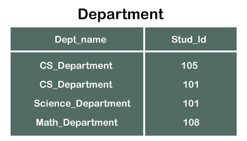
Consider two tables Student and Department having their respective attributes as shown in the below table structure:

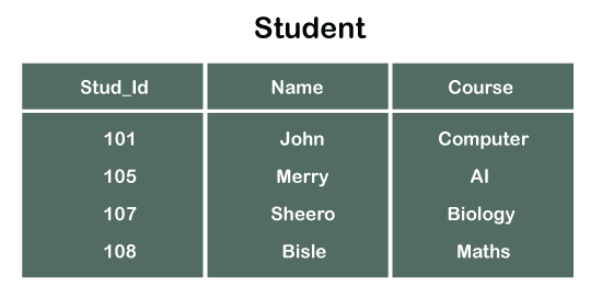
In the tables, one attribute, you can see, is common, that is Stud_Id, but it has different key constraints for both tables. In the Student table, the field Stud_Id is a primary key because it is uniquely identifying all other fields of the Student table. On the other hand, Stud_Id is a foreign key attribute for the Department table because it is acting as a primary key attribute for the Student table. It means that both the Student and Department table are linked with one another because of the Stud_Id attribute.

In the below-shown figure, you can view the following structure of the relationship between the two tables.

Note: Referential Integrity in DBMS is developed from the concept of the foreign key. It is clear that a primary key is an alone existing key and a foreign key always reference to a primary key in some other table, in which the table that contains the primary key is known as the referenced table or parent table for the other table that is having the foreign key.

Q5) Create Foreign Key constraint with an example?

A5)

On CREATE TABLE

Below is the syntax that will make us learn the creation of a foreign key in a table:

1. CREATE TABLE Department (  
2.    Dept_name varchar (120) NOT NULL,  
3.    Stud_Id int,  
4.      FOREIGN KEY (Stud_Id) REFERENCES Student (Stud_Id)  
5. );  

So, in this way, we can set a foreign key for a table in the MYSQL database.

In case of creating a foreign key for a table in SQL or Oracle server, the following syntax will work:

1. CREATE TABLE Department (  
2.    Dept_name varchar (120) NOT NULL,  
3.    Stud_Id int FOREIGN KEY REFERENCES Student (Stud_Id)  
4. );  

On ALTER TABLE

Following is the syntax for creating a foreign key constraint on ALTER TABLE:

1. ALTER TABLE Department  
2. ADD FOREIGN KEY (Stud_Id) REFERENCES Student (Stud_Id);  

Q6) What is relational algebra and what are its types give examples also?

A6) Relational algebra is a procedural query language. It gives a step by step process to obtain the result of the query. It uses operators to perform queries.

Types of Relational operation

Fig 3 - Relational operation

1. Select Operation:

●        The select operation selects tuples that satisfy a given predicate.

●        It is denoted by sigma (σ).

Notation:  σ p(r)  

Where:

σ is used for selection prediction

r is used for relation

p is used as a propositional logic formula which may use connectors like: AND OR

And NOT. These relational can use as relational operators like =, ≠, ≥, <, >, ≤.

For example: LOAN Relation

Input:

1. σ BRANCH_NAME="perryride" (LOAN)  

Output:

2. Project Operation:

●        This operation shows the list of those attributes that we wish to appear in the result. Rest of the attributes are eliminated from the table.

●        It is denoted by ∏.

Notation: ∏ A1, A2, An (r)   

Where

A1, A2, A3 is used as an attribute name of relation r.

Example: CUSTOMER RELATION

Input:

1. ∏ NAME, CITY (CUSTOMER)  

Output:

3. Union Operation:

●        Suppose there are two tuples R and S. The union operation contains all the tuples that are either in R or S or both in R & S.

●        It eliminates the duplicate tuples. It is denoted by ∪.

Notation: R ∪ S   

A union operation must hold the following condition:

●        R and S must have the attribute of the same number.

●        Duplicate tuples are eliminated automatically.

Example:

DEPOSITOR RELATION

BORROW RELATION

Input:

1. ∏ CUSTOMER_NAME (BORROW) ∪ ∏ CUSTOMER_NAME (DEPOSITOR)  

Output:

4. Set Intersection:

●        Suppose there are two tuples R and S. The set intersection operation contains all tuples that are in both R & S.

●        It is denoted by intersection ∩.

Notation: R ∩ S   

Example: Using the above DEPOSITOR table and BORROW table

Input:

1. ∏ CUSTOMER_NAME (BORROW) ∩ ∏ CUSTOMER_NAME (DEPOSITOR)  

Output:

5. Set Difference:

●        Suppose there are two tuples R and S. The set intersection operation contains all tuples that are in R but not in S.

●        It is denoted by intersection minus (-).

Notation: R - S  

Example: Using the above DEPOSITOR table and BORROW table

Input:

1. ∏ CUSTOMER_NAME (BORROW) - ∏ CUSTOMER_NAME (DEPOSITOR)  

Output:

6. Cartesian product

●        The Cartesian product is used to combine each row in one table with each row in the other table. It is also known as a cross product.

●        It is denoted by X.

Notation: E X D  

Example:

EMPLOYEE

DEPARTMENT

Input:

1. EMPLOYEE X DEPARTMENT  

Output:

7. Rename Operation:

The rename operation is used to rename the output relation. It is denoted by rho (ρ).

Example: We can use the rename operator to rename STUDENT relation to STUDENT1.

ρ(STUDENT1, STUDENT)  

Q7) Explain join operation and its different types with examples?

A7) A Join operation combines related tuples from different relations, if and only if a given join condition is satisfied. It is denoted by ⋈.

Example:

EMPLOYEE

SALARY

1. Operation: (EMPLOYEE ⋈ SALARY)   

Result:

Types of Join operations:

Fig 4 – Join Operation

1. Natural Join:

●        A natural join is the set of tuples of all combinations in R and S that are equal on their common attribute names.

●        It is denoted by ⋈.

Example: Let's use the above EMPLOYEE table and SALARY table:

Input:

1. ∏EMP_NAME, SALARY (EMPLOYEE ⋈ SALARY)  

Output:

2. Outer Join:

The outer join operation is an extension of the join operation. It is used to deal with missing information.

Example:

EMPLOYEE

FACT_WORKERS

Input:

1. (EMPLOYEE ⋈ FACT_WORKERS)  

Output:

An outer join is basically of three types:

1. Left outer join
2. Right outer join
3. Full outer join

a. Left outer join:

●        Left outer join contains the set of tuples of all combinations in R and S that are equal on their common attribute names.

●        In the left outer join, tuples in R have no matching tuples in S.

●        It is denoted by ⟕.

Example: Using the above EMPLOYEE table and FACT_WORKERS table

Input:

1. EMPLOYEE ⟕ FACT_WORKERS   

b. Right outer join:

●        Right outer join contains the set of tuples of all combinations in R and S that are equal on their common attribute names.

●        In right outer join, tuples in S have no matching tuples in R.

●        It is denoted by ⟖.

Example: Using the above EMPLOYEE table and FACT_WORKERS Relation

Input:

1. EMPLOYEE ⟖ FACT_WORKERS  

Output:

c. Full outer join:

●        Full outer join is like a left or right join except that it contains all rows from both tables.

●        In full outer join, tuples in R that have no matching tuples in S and tuples in S that have no matching tuples in R in their common attribute name.

●        It is denoted by ⟗.

Example: Using the above EMPLOYEE table and FACT_WORKERS table

Input:

1. EMPLOYEE ⟗ FACT_WORKERS  

Output:

3. Equijoin:

It is also known as an inner join. It is the most common join. It is based on matched data as per the equality condition. The equi join uses the comparison operator(=).

Example:

CUSTOMER RELATION

PRODUCT

Input:

1. CUSTOMER ⋈ PRODUCT    

Output:

Q8) What is relational calculus and what are its types explain with examples?

A8) Relational Calculus

●        Relational calculus is a non-procedural query language. In the non-procedural query language, the user is concerned with the details of how to obtain the end results.

●        The relational calculus tells what to do but never explains how to do.

Types of Relational calculus:

Fig 5 - Relational calculus

1. Tuple Relational Calculus (TRC)

●        The tuple relational calculus is specified to select the tuples in a relation. In TRC, filtering variable uses the tuples of a relation.

●        The result of the relation can have one or more tuples.

Notation:

1. {T | P (T)}   or {T | Condition (T)}   

Where

T is the resulting tuples

P(T) is the condition used to fetch T.

For example:

1. { T.name | Author(T) AND T.article = 'database' }  

OUTPUT: This query selects the tuples from the AUTHOR relation. It returns a tuple with 'name' from Author who has written an article on 'database'.

TRC (tuple relation calculus) can be quantified. In TRC, we can use Existential (∃) and Universal Quantifiers (∀).

For example:

1. { R| ∃T ∈ Authors(T.article='database' AND R.name=T.name)}  

Output: This query will yield the same result as the previous one.

2. Domain Relational Calculus (DRC)

●        The second form of relation is known as Domain relational calculus. In domain relational calculus, filtering variable uses the domain of attributes.

●        Domain relational calculus uses the same operators as tuple calculus. It uses logical connectives ∧ (and), ∨ (or) and ┓ (not).

●        It uses Existential (∃) and Universal Quantifiers (∀) to bind the variable.

Notation:

1. { a1, a2, a3, ..., an | P (a1, a2, a3, ... ,an)}  

Where

a1, a2 are attributes

P stands for formula built by inner attributes

For example:

1. {< article, page, subject > |  ∈ javatpoint ∧ subject = 'database'}  

Output: This query will yield the article, page, and subject from the relational javatpoint, where the subject is a database.

Q9) What are keys in DBMS and explain different types of keys.

A9)

Keys are the entity's attributes, which define the entity's record uniquely.

Several types of keys exist.

These are listed underneath:

❏      Composite key

A composite key consists of two attributes or more, but it must be minimal.

❏      Candidate key

A candidate key is a key that is simple or composite and special and minimal. It is special since no two rows can have the same value at any time in a table. It is minimal since, in order to achieve uniqueness, every column is required.

❏      Super key

The Super Key is one or more of the entity's attributes that uniquely define the database record.

❏      Primary key

The primary key is a candidate key that the database designer chooses to be used as an identification mechanism for the entire set of entities. In a table, it must uniquely classify tuples and not be null.

In the ER model, the primary key is indicated by underlining the attribute.

●      To uniquely recognise tuples in a table, the designer selects a candidate key. It must not be empty.

●      A key is selected by the database builder to be used by the entire entity collection as an authentication mechanism. This is regarded as the primary key. In the ER model, this key is indicated by underlining the attribute.

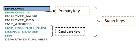
Fig 6: Shows different keys

❏      Alternate key

Alternate keys are all candidate keys not chosen as the primary key.

❏      Foreign key

A foreign key (FK) is an attribute in a table that, in another table, references the primary key OR it may be null. The same data type must be used for both international and primary keys.

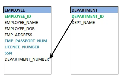
Fig 7: Foreign key

❏      Secondary key

A secondary key is an attribute used exclusively (can be composite) for retrieval purposes, such as: phone and last name.

Q10) What is relational algebra and what operations can be performed using relational algebra?

A10)

Relational Algebra is procedural query language. It takes Relation as input and generates relation as output. Relational algebra mainly provides theoretical foundation for relational databases and SQL.

Basic Operations which can be performed using relational algebra are:

1. Projection

2. Selection

3. Join

4. Union

5. Set Difference

6. Intersection

7. Cartesian product

8. Rename

Q11) Write about Projection, Selection and Join operations of relational algebra.

A11)

Consider following relation R (A, B, C)

1. Projection (π):

This operation is used to select particular columns from the relation.

Π(AB) R:

It will select A and B column from the relation R. It produces the output like:

Project operation automatically removes duplicates from the resultant set.

2. Selection (σ):

This operation is used to select particular tuples from the relation.

σ(C<4) R:

It will select the tuples which have a value of c less than 4.

But select operation is used to only select the required tuples from the relation. To display those tuples on screen, select operation must be combined with project operation.

Π (σ (C<4) R) will produce the result like:

3. Join 

A Cartesian product followed by a selection criterion is basically a joint process.

Operation of join, denoted by ⋈.

The JOIN operation often allows tuples from different relationships to join different tuples

Types of JOIN:

Various forms of join operation are:

Inner Joins:

• Theta join
• EQUI join
• Natural join

Outer join:

• Left Outer Join
• Right Outer Join
• Full Outer Join

Q12) Write about Union, Set Difference and Intersection operations of relational algebra.

A12)

Union

Union operation in relational algebra is the same as union operation in set theory, only the restriction is that both relations must have the same set of attributes for a union of two relationships.

Syntax:  table_name1 ∪ table_name2

For instance, if we have two tables with RegularClass and ExtraClass, both have a student column to save the student name, then,

∏Student(RegularClass) ∪ ∏Student(ExtraClass)

The above operation will send us the names of students who attend both normal and extra classes, reducing repetition.

Set difference

Set Difference in relational algebra is the same operation of set difference as in set theory, with the limitation that the same set of attributes can have both relationships.

Syntax: A - B

Where the A and B relationships.

For instance, if we want to find the names of students who attend the regular class, but not the extra class, then we can use the following procedure:

∏Student(RegularClass) - ∏Student(ExtraClass)

Intersection

The symbol ∩ is the definition of an intersection.

A ∩ B

Defines a relationship consisting of a set of all the tuples in both A and B. A and B must be union-compatible, however.

Q13) Write about Cartesian product and rename operations of relational algebra.

A13)

Cartesian product

This is used to merge information into one from two separate relationships(tables) and to fetch information from the merged relationship.

Syntax: A X B

For example, if we want to find the morning Regular Class and Extra Class data, then we can use the following operation:

σtime = 'morning' (RegularClass X ExtraClass)

Both RegularClass and ExtraClass should have the attribute time for the above query to operate.

Rename

Rename is a unified operation that is used to rename relationship attributes.

ρ (a/b)R renames the 'b' component of the partnership to 'a'.

Syntax: ρ(RelationNew, RelationOld)

Unit - 2

Relational Data Model

Q1) Explain in brief relational data model?

A1) Relational data model is the primary data model, which is used widely around the world for data storage and processing. This model is simple and it has all the properties and capabilities required to process data with storage efficiency.

Concepts

Tables−In relational data model, relations are saved in the format of Tables. This format stores the relation among entities. A table has rows and columns, where rows represents records and columns represent the attributes.

Tuple− A single row of a table, which contains a single record for that relation is called a tuple.

Relation instance− A finite set of tuples in the relational database system represents relation instance. Relation instances do not have duplicate tuples.

Relation schema− A relation schema describes the relation name (table name), attributes, and their names.

Relation key−Each row has one or more attributes, known as relation key, which can identify the row in the relation (table) uniquely.

Attribute domain−Every attribute has some predefined value scope, known as attribute domain.

Constraints

Every relation has some conditions that must hold for it to be a valid relation. These conditions are called Relational Integrity Constraints. There are three main integrity constraints −

●        Key constraints

●        Domain constraints

●        Referential integrity constraints

Key Constraints

There must be at least one minimal subset of attributes in the relation, which can identify a tuple uniquely. This minimal subset of attributes is called key for that relation. If there are more than one such minimal subsets, these are called candidate keys.

Key constraints force that −

• In a relation with a key attribute, no two tuples can have identical values for key attributes.
• A key attribute cannot have NULL values
• Key constraints are also referred to as Entity Constraints.

Domain Constraints

Attributes have specific values in real-world scenario. For example, age can only be a positive integer. The same constraints have been tried to employ on the attributes of a relation. Every attribute is bound to have a specific range of values. For example, age cannot be less than zero and telephone numbers cannot contain a digit outside 0-9.

Referential integrity Constraints

Referential integrity constraints work on the concept of Foreign Keys. A foreign key is a key attribute of a relation that can be referred in other relation.

Referential integrity constraint states that if a relation refers to a key attribute of a different or same relation, then that key element must exist.

Q2) Write short notes on database schema and database instance?

A2) Database Schema

A database schema is the skeleton structure that represents the logical view of the entire database. It defines how the data is organized and how the relations among them are associated. It formulates all the constraints that are to be applied on the data.

A database schema defines its entities and the relationship among them. It contains a descriptive detail of the database, which can be depicted by means of schema diagrams. It’s the database designers who design the schema to help programmers understand the database and make it useful.

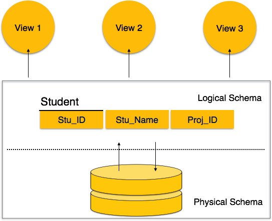
Fig 1 - Database schema

A database schema can be divided broadly into two categories −

●        Physical Database Schema−This schema pertains to the actual storage of data and its form of storage like files, indices, etc. It defines how the data will be stored in a secondary storage.

●        Logical Database Schema−This schema defines all the logical constraints that need to be applied on the data stored. It defines tables, views, and integrity constraints.

Database Instance

It is important that we distinguish these two terms individually. Database schema is the skeleton of database. It is designed when the database doesn't exist at all. Once the database is operational, it is very difficult to make any changes to it. A database schema does not contain any data or information.

A database instance is a state of operational database with data at any given time. It contains a snapshot of the database. Database instances tend to change with time. A DBMS ensures that its every instance (state) is in a valid state, by diligently following all the validations, constraints, and conditions that the database designers have imposed.

Q3) Explain in brief integrity constraints?

A3) Integrity Constraints

●        Integrity constraints are a set of rules. It is used to maintain the quality of information.

●        Integrity constraints ensure that the data insertion, updating, and other processes have to be performed in such a way that data integrity is not affected.

●        Thus, integrity constraint is used to guard against accidental damage to the database.

Types of Integrity Constraint

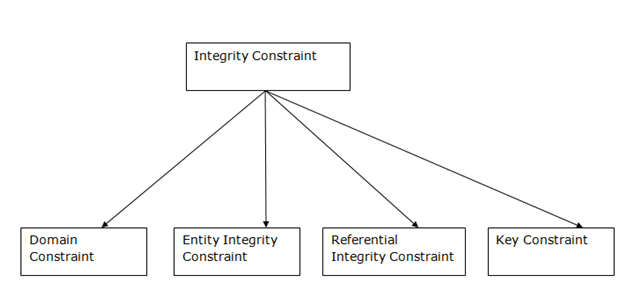
Fig 2 - Integrity Constraint

1. Domain constraints

●        Domain constraints can be defined as the definition of a valid set of values for an attribute.

●        The data type of domain includes string, character, integer, time, date, currency, etc. The value of the attribute must be available in the corresponding domain.

Example:

2. Entity integrity constraints

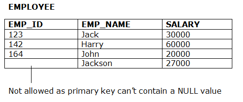
●        The entity integrity constraint states that primary key value can't be null.

●        This is because the primary key value is used to identify individual rows in relation and if the primary key has a null value, then we can't identify those rows.

●        A table can contain a null value other than the primary key field.

Example:

3. Referential Integrity Constraints

●        A referential integrity constraint is specified between two tables.

●        In the Referential integrity constraints, if a foreign key in Table 1 refers to the Primary Key of Table 2, then every value of the Foreign Key in Table 1 must be null or be available in Table 2.

Example:

4. Key constraints

●        Keys are the entity set that is used to identify an entity within its entity set uniquely.

●        An entity set can have multiple keys, but out of which one key will be the primary key. A primary key can contain a unique and null value in the relational table.

Example:

Q4) What is Foreign Key in DBMS?

A4) Foreign key

A foreign key is different from a super key, candidate key or primary key because a foreign key is the one that is used to link two tables together or create connectivity between the two.

Here, in this section, we will discuss foreign key, its use and look at some examples that will help us to understand the working and use of the foreign key. We will also see its practical implementation on a database, i.e., creating and deleting a foreign key on a table.

What is a Foreign Key

A foreign key is the one that is used to link two tables together via the primary key. It means the columns of one table points to the primary key attribute of the other table. It further means that if any attribute is set as a primary key attribute will work in another table as a foreign key attribute. But one should know that a foreign key has nothing to do with the primary key.

Use of Foreign Key

The use of a foreign key is simply to link the attributes of two tables together with the help of a primary key attribute. Thus, it is used for creating and maintaining the relationship between the two relations.

Example of Foreign Key

Let's discuss an example to understand the working of a foreign key.

Consider two tables Student and Department having their respective attributes as shown in the below table structure:

In the tables, one attribute, you can see, is common, that is Stud_Id, but it has different key constraints for both tables. In the Student table, the field Stud_Id is a primary key because it is uniquely identifying all other fields of the Student table. On the other hand, Stud_Id is a foreign key attribute for the Department table because it is acting as a primary key attribute for the Student table. It means that both the Student and Department table are linked with one another because of the Stud_Id attribute.

In the below-shown figure, you can view the following structure of the relationship between the two tables.

Note: Referential Integrity in DBMS is developed from the concept of the foreign key. It is clear that a primary key is an alone existing key and a foreign key always reference to a primary key in some other table, in which the table that contains the primary key is known as the referenced table or parent table for the other table that is having the foreign key.

Q5) Create Foreign Key constraint with an example?

A5)

On CREATE TABLE

Below is the syntax that will make us learn the creation of a foreign key in a table:

1. CREATE TABLE Department (  
2.    Dept_name varchar (120) NOT NULL,  
3.    Stud_Id int,  
4.      FOREIGN KEY (Stud_Id) REFERENCES Student (Stud_Id)  
5. );  

So, in this way, we can set a foreign key for a table in the MYSQL database.

In case of creating a foreign key for a table in SQL or Oracle server, the following syntax will work:

1. CREATE TABLE Department (  
2.    Dept_name varchar (120) NOT NULL,  
3.    Stud_Id int FOREIGN KEY REFERENCES Student (Stud_Id)  
4. );  

On ALTER TABLE

Following is the syntax for creating a foreign key constraint on ALTER TABLE:

1. ALTER TABLE Department  
2. ADD FOREIGN KEY (Stud_Id) REFERENCES Student (Stud_Id);  

Q6) What is relational algebra and what are its types give examples also?

A6) Relational algebra is a procedural query language. It gives a step by step process to obtain the result of the query. It uses operators to perform queries.

Types of Relational operation

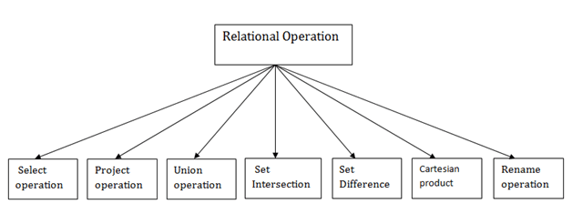
Fig 3 - Relational operation

1. Select Operation:

●        The select operation selects tuples that satisfy a given predicate.

●        It is denoted by sigma (σ).

Notation:  σ p(r)  

Where:

σ is used for selection prediction

r is used for relation

p is used as a propositional logic formula which may use connectors like: AND OR

And NOT. These relational can use as relational operators like =, ≠, ≥, <, >, ≤.

For example: LOAN Relation

Input:

1. σ BRANCH_NAME="perryride" (LOAN)  

Output:

2. Project Operation:

●        This operation shows the list of those attributes that we wish to appear in the result. Rest of the attributes are eliminated from the table.

●        It is denoted by ∏.

Notation: ∏ A1, A2, An (r)   

Where

A1, A2, A3 is used as an attribute name of relation r.

Example: CUSTOMER RELATION

Input:

1. ∏ NAME, CITY (CUSTOMER)  

Output:

3. Union Operation:

●        Suppose there are two tuples R and S. The union operation contains all the tuples that are either in R or S or both in R & S.

●        It eliminates the duplicate tuples. It is denoted by ∪.

Notation: R ∪ S   

A union operation must hold the following condition:

●        R and S must have the attribute of the same number.

●        Duplicate tuples are eliminated automatically.

Example:

DEPOSITOR RELATION

BORROW RELATION

Input:

1. ∏ CUSTOMER_NAME (BORROW) ∪ ∏ CUSTOMER_NAME (DEPOSITOR)  

Output:

4. Set Intersection:

●        Suppose there are two tuples R and S. The set intersection operation contains all tuples that are in both R & S.

●        It is denoted by intersection ∩.

Notation: R ∩ S   

Example: Using the above DEPOSITOR table and BORROW table

Input:

1. ∏ CUSTOMER_NAME (BORROW) ∩ ∏ CUSTOMER_NAME (DEPOSITOR)  

Output:

5. Set Difference:

●        Suppose there are two tuples R and S. The set intersection operation contains all tuples that are in R but not in S.

●        It is denoted by intersection minus (-).

Notation: R - S  

Example: Using the above DEPOSITOR table and BORROW table

Input:

1. ∏ CUSTOMER_NAME (BORROW) - ∏ CUSTOMER_NAME (DEPOSITOR)  

Output:

6. Cartesian product

●        The Cartesian product is used to combine each row in one table with each row in the other table. It is also known as a cross product.

●        It is denoted by X.

Notation: E X D  

Example:

EMPLOYEE

DEPARTMENT

Input:

1. EMPLOYEE X DEPARTMENT  

Output:

7. Rename Operation:

The rename operation is used to rename the output relation. It is denoted by rho (ρ).

Example: We can use the rename operator to rename STUDENT relation to STUDENT1.

ρ(STUDENT1, STUDENT)  

Q7) Explain join operation and its different types with examples?

A7) A Join operation combines related tuples from different relations, if and only if a given join condition is satisfied. It is denoted by ⋈.

Example:

EMPLOYEE

SALARY

1. Operation: (EMPLOYEE ⋈ SALARY)   

Result:

Types of Join operations:

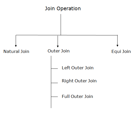
Fig 4 – Join Operation

1. Natural Join:

●        A natural join is the set of tuples of all combinations in R and S that are equal on their common attribute names.

●        It is denoted by ⋈.

Example: Let's use the above EMPLOYEE table and SALARY table:

Input:

1. ∏EMP_NAME, SALARY (EMPLOYEE ⋈ SALARY)  

Output:

2. Outer Join:

The outer join operation is an extension of the join operation. It is used to deal with missing information.

Example:

EMPLOYEE

FACT_WORKERS

Input:

1. (EMPLOYEE ⋈ FACT_WORKERS)  

Output:

An outer join is basically of three types:

1. Left outer join
2. Right outer join
3. Full outer join

a. Left outer join:

●        Left outer join contains the set of tuples of all combinations in R and S that are equal on their common attribute names.

●        In the left outer join, tuples in R have no matching tuples in S.

●        It is denoted by ⟕.

Example: Using the above EMPLOYEE table and FACT_WORKERS table

Input:

1. EMPLOYEE ⟕ FACT_WORKERS   

b. Right outer join:

●        Right outer join contains the set of tuples of all combinations in R and S that are equal on their common attribute names.

●        In right outer join, tuples in S have no matching tuples in R.

●        It is denoted by ⟖.

Example: Using the above EMPLOYEE table and FACT_WORKERS Relation

Input:

1. EMPLOYEE ⟖ FACT_WORKERS  

Output:

c. Full outer join:

●        Full outer join is like a left or right join except that it contains all rows from both tables.

●        In full outer join, tuples in R that have no matching tuples in S and tuples in S that have no matching tuples in R in their common attribute name.

●        It is denoted by ⟗.

Example: Using the above EMPLOYEE table and FACT_WORKERS table

Input:

1. EMPLOYEE ⟗ FACT_WORKERS  

Output:

3. Equijoin:

It is also known as an inner join. It is the most common join. It is based on matched data as per the equality condition. The equi join uses the comparison operator(=).

Example:

CUSTOMER RELATION

PRODUCT

Input:

1. CUSTOMER ⋈ PRODUCT    

Output:

Q8) What is relational calculus and what are its types explain with examples?

A8) Relational Calculus

●        Relational calculus is a non-procedural query language. In the non-procedural query language, the user is concerned with the details of how to obtain the end results.

●        The relational calculus tells what to do but never explains how to do.

Types of Relational calculus:

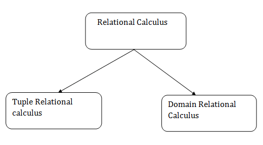
Fig 5 - Relational calculus

1. Tuple Relational Calculus (TRC)

●        The tuple relational calculus is specified to select the tuples in a relation. In TRC, filtering variable uses the tuples of a relation.

●        The result of the relation can have one or more tuples.

Notation:

1. {T | P (T)}   or {T | Condition (T)}   

Where

T is the resulting tuples

P(T) is the condition used to fetch T.

For example:

1. { T.name | Author(T) AND T.article = 'database' }  

OUTPUT: This query selects the tuples from the AUTHOR relation. It returns a tuple with 'name' from Author who has written an article on 'database'.

TRC (tuple relation calculus) can be quantified. In TRC, we can use Existential (∃) and Universal Quantifiers (∀).

For example:

1. { R| ∃T ∈ Authors(T.article='database' AND R.name=T.name)}  

Output: This query will yield the same result as the previous one.

2. Domain Relational Calculus (DRC)

●        The second form of relation is known as Domain relational calculus. In domain relational calculus, filtering variable uses the domain of attributes.

●        Domain relational calculus uses the same operators as tuple calculus. It uses logical connectives ∧ (and), ∨ (or) and ┓ (not).

●        It uses Existential (∃) and Universal Quantifiers (∀) to bind the variable.

Notation:

1. { a1, a2, a3, ..., an | P (a1, a2, a3, ... ,an)}  

Where

a1, a2 are attributes

P stands for formula built by inner attributes

For example:

1. {< article, page, subject > |  ∈ javatpoint ∧ subject = 'database'}  

Output: This query will yield the article, page, and subject from the relational javatpoint, where the subject is a database.

Q9) What are keys in DBMS and explain different types of keys.

A9)

Keys are the entity's attributes, which define the entity's record uniquely.

Several types of keys exist.

These are listed underneath:

❏      Composite key

A composite key consists of two attributes or more, but it must be minimal.

❏      Candidate key

A candidate key is a key that is simple or composite and special and minimal. It is special since no two rows can have the same value at any time in a table. It is minimal since, in order to achieve uniqueness, every column is required.

❏      Super key

The Super Key is one or more of the entity's attributes that uniquely define the database record.

❏      Primary key

The primary key is a candidate key that the database designer chooses to be used as an identification mechanism for the entire set of entities. In a table, it must uniquely classify tuples and not be null.

In the ER model, the primary key is indicated by underlining the attribute.

●      To uniquely recognise tuples in a table, the designer selects a candidate key. It must not be empty.

●      A key is selected by the database builder to be used by the entire entity collection as an authentication mechanism. This is regarded as the primary key. In the ER model, this key is indicated by underlining the attribute.

Fig 6: Shows different keys

❏      Alternate key

Alternate keys are all candidate keys not chosen as the primary key.

❏      Foreign key

A foreign key (FK) is an attribute in a table that, in another table, references the primary key OR it may be null. The same data type must be used for both international and primary keys.

Fig 7: Foreign key

❏      Secondary key

A secondary key is an attribute used exclusively (can be composite) for retrieval purposes, such as: phone and last name.

Q10) What is relational algebra and what operations can be performed using relational algebra?

A10)

Relational Algebra is procedural query language. It takes Relation as input and generates relation as output. Relational algebra mainly provides theoretical foundation for relational databases and SQL.

Basic Operations which can be performed using relational algebra are:

1. Projection

2. Selection

3. Join

4. Union

5. Set Difference

6. Intersection

7. Cartesian product

8. Rename

Q11) Write about Projection, Selection and Join operations of relational algebra.

A11)

Consider following relation R (A, B, C)

1. Projection (π):

This operation is used to select particular columns from the relation.

Π(AB) R:

It will select A and B column from the relation R. It produces the output like:

Project operation automatically removes duplicates from the resultant set.

2. Selection (σ):

This operation is used to select particular tuples from the relation.

σ(C<4) R:

It will select the tuples which have a value of c less than 4.

But select operation is used to only select the required tuples from the relation. To display those tuples on screen, select operation must be combined with project operation.

Π (σ (C<4) R) will produce the result like:

3. Join 

A Cartesian product followed by a selection criterion is basically a joint process.

Operation of join, denoted by ⋈.

The JOIN operation often allows tuples from different relationships to join different tuples

Types of JOIN:

Various forms of join operation are:

Inner Joins:

• Theta join
• EQUI join
• Natural join

Outer join:

• Left Outer Join
• Right Outer Join
• Full Outer Join

Q12) Write about Union, Set Difference and Intersection operations of relational algebra.

A12)

Union

Union operation in relational algebra is the same as union operation in set theory, only the restriction is that both relations must have the same set of attributes for a union of two relationships.

Syntax:  table_name1 ∪ table_name2

For instance, if we have two tables with RegularClass and ExtraClass, both have a student column to save the student name, then,

∏Student(RegularClass) ∪ ∏Student(ExtraClass)

The above operation will send us the names of students who attend both normal and extra classes, reducing repetition.

Set difference

Set Difference in relational algebra is the same operation of set difference as in set theory, with the limitation that the same set of attributes can have both relationships.

Syntax: A - B

Where the A and B relationships.

For instance, if we want to find the names of students who attend the regular class, but not the extra class, then we can use the following procedure:

∏Student(RegularClass) - ∏Student(ExtraClass)

Intersection

The symbol ∩ is the definition of an intersection.

A ∩ B

Defines a relationship consisting of a set of all the tuples in both A and B. A and B must be union-compatible, however.

Q13) Write about Cartesian product and rename operations of relational algebra.

A13)

Cartesian product

This is used to merge information into one from two separate relationships(tables) and to fetch information from the merged relationship.

Syntax: A X B

For example, if we want to find the morning Regular Class and Extra Class data, then we can use the following operation:

σtime = 'morning' (RegularClass X ExtraClass)

Both RegularClass and ExtraClass should have the attribute time for the above query to operate.

Rename

Rename is a unified operation that is used to rename relationship attributes.

ρ (a/b)R renames the 'b' component of the partnership to 'a'.

Syntax: ρ(RelationNew, RelationOld)