Unit - 6

Statistics and finite differences

Q1) Find the best values of a and b so that y = a + bx fits the data given in the table

A1)

y = a + bx

x	y	Xy
0	1.0	0	0
1	2.9	2.0	1
2	4.8	9.6	4
3	6.7	20.1	9
4	8.6	13.4	16
x = 10	y ,= 24.0	xy = 67.0

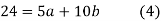
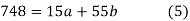
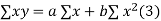
Normal equations, y= na+ bx  (2)

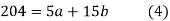
On putting the values of

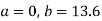
On solving (4) and (5) we get,

On substituting the values of a and b in (1) we get

Q2) By the method of least squares, find the straight line that best fits the following data )

A2)

Let the equation of the straight line best fit be y = a + bx.     (1)

x	y	x y
1	14	14	1
2	27	54	4
3	40	120	9
4	55	220	16
5	68	340	25
x=15	y=204	xy=748

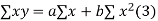
Normal equations are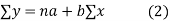

On putting the values of x, y, xy and in (2) and (3) we have

On solving equations (4) and (5) we get

On substituting the values of (a) and (b) in (1) we get,

Q3) Find the least squares approximation of second degree for the discrete data

A3)

Let the equation of second degree polynomial be

x	y	Xy
-2	15	-30	4	60	-8	16
-1	1	-1	1	1	-1	1
0	1	0	0	0	0	0
1	3	3	1	3	1	1
2	19	38	4	76	8	16
x=0	y=39	xy=10

Normal equations are

On putting the values of x, y, xy,

have

On solving (5),(6),(7), we get,

The required polynomial of second degree is

Q4) Fit a second degree parabola to the following data by least square method:

A4)

Taking

Taking

The equation is transformed to

x		y		Uv
1929	-4	352	-5	20	16	-80	-64	256
1930	-3	360	-1	3	9	-9	-27	81
1931	-2	357	0	0	4	0	-8	16
1932	-1	358	1	-1	1	1	-1	1
1933	0	360	3	0	0	0	0	0
1934	1	361	4	4	1	4	1	1
1935	2	361	4	8	4	16	8	16
1936	3	360	3	9	9	27	27	81
1937	4	350	2	8	16	32	64	256
Total	u=0		y=11	uv=51

Normal equations are

On solving these equations we get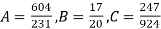

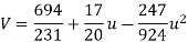
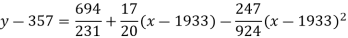
Q5) Find the least squares approximation of second degree for the discrete data

A5)

Let the equation of second degree polynomial be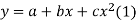

x	y	Xy
-2	15	-30	4	60	-8	16
-1	1	-1	1	1	-1	1
0	1	0	0	0	0	0
1	3	3	1	3	1	1
2	19	38	4	76	8	16
x=0	y=39	xy=10

Normal equations are

On putting the values of x, y, xy,

have

On solving (5),(6),(7), we get,

The required polynomial of second degree is

Q6) Fit a second degree parabola to the following data.

A6)

We shift the origin to (2.5, 0) antique 0.5 as the new unit. This amounts to changing the variable x to X, by the relation X = 2x – 5.

Let the parabola of fit be y = a + bXThe values of X etc. Are calculated as below:

x	X	y	Xy
1.0	-3	1.1	-3.3	9	9.9	-27	81
1.5	-2	1.3	-2.6	4	5.2	-5	16
2.0	-1	1.6	-1.6	1	1.6	-1	1
2.5	0	2.0	0.0	0	0.0	0	0
3.0	1	2.7	2.7	1	2.7	1	1
3.5	2	3.4	6.8	4	13.6	8	16
4.0	3	4.1	12.3	9	36.9	27	81
Total	0	16.2	14.3	28	69.9	0	196

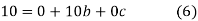
The normal equations are

7a + 28c =16.2; 28b =14.3;. 28a +196c=69.9

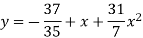
Solving these as simultaneous equations we get

Replacing X bye 2x – 5 in the above equation we get

Which simplifies to y =

This is the required parabola of the best fit.

Q7) Estimate the chlorine residual in a swimming pool 5 hours after it has been treated with chemicals by fitting an exponential curve of the form

of the data given below-

A7)

Taking log on the curve which is non-linear,

We get-

Put

Then-

Which is the linear equation in X,

Its nomal equations are-

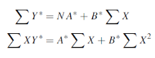
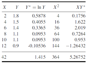
Here N = 6,

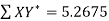
Thus the normal equations are-

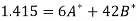
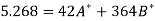
On solving, we get

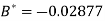
Or

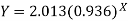
A = 2.013 and B = 0.936

Hence the required least square exponential curve-

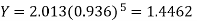
Prediction-

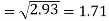
Chlorine content after 5 hours-

Q8) What do you understand by positive correlation and negative correlation?

A8)

Positive Correlation:

Correlation between two variables is said to be positive if the values of thevariables deviate in the same direction i.e. if the values of one variable increase (or decrease) then the values of other variable also increase (or decrease). For example:

1. Heights and weights of group of persons;

2. House hold income and expenditure;

3. Amount of rainfall and yield of crops

Negative Correlation:

Correlation between two variables is said to be negative if the values of variables deviate in opposite direction i.e. if the values of one variable increase (or decrease) then the values of other variable decrease (or increase). Some examples of negative correlations are correlation between

1. Volume and pressure of perfect gas;

2. Price and demand of goods;

3. Literacy and poverty in a country

Q9) What is Karl Pearson’s coefficient of correlation?

A9)

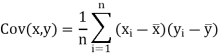
Coefficient of correlation measures the intensity or degree of linear relationship between two variables. It was given by British Biometrician Karl Pearson (1867-1936).

Karl Pearson’s Coefficient of Correlation is widely used mathematical method is used to calculate the degree and direction of the relationship between linear related variables. The coefficient of correlation is denoted by “r”.

If X and Y are two random variables then correlation coefficient between X and Y is denoted by r and defined as-

Karl Pearson’s coefficient of correlation-

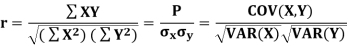
Here- and

Q10) Find the correlation coefficient between Age and weight of the following data-

A10)

x	Y					( ) )
30	56	-10	100	-4	16	40
44	55	4	16	-5	25	-20
45	60	5	25	0	0	0
43	64	3	9	4	16	12
34	62	-6	36	2	4	-12
44	63	4	16	3	9	12
Sum= 240	360	0	202	0	70	32

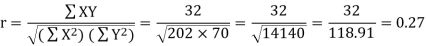
Karl Pearson’s coefficient of correlation-

Q11) Find the correlation coefficient between the values X and Y of the dataset given below by using short-cut method-

A11)

X	Y
10	90	-20	400	20	400	-400
20	85	-10	100	15	225	-150
30	80	0	0	10	100	0
40	60	10	100	-10	100	-100
50	45	20	400	-25	625	-500
Sum = 150	360	0	1000	10	1450	-1150

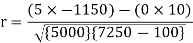
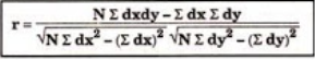
Short-cut method to calculate correlation coefficient-

Q12) Psychological tests of intelligence and of engineering ability were applied to 10 students. Here is a record of ungrouped data showing intelligence ratio (I.R) and engineering ratio (E.R). Calculate the co-efficient of correlation.

A12)

We construct the following table:

Student	Intelligence ratio	Engineering ratio
A B C D E F G H I J	100                      6     104                     5     102                     3     101                     2     100                     1       99                     0       98                    -1       96                    -3       93                    -6       92                    -7	101                 3   103                 5   100                 2    98                  0    95                 -3    96                 -2   104                 6    92                 -6    97                 -1    94                 -4	36 25 9 4 1 0 1 9 36 49	9 25 4 0 9 4 36 36 1 16	18 25 6 0 -3 0 -6 18 6 28
Total	990                    0	980                 0	170	140	92

From this table, mean of i.e., and mean of , i.e.,

Substituting these values in the formula (1), we have

Q13) Calculate coefficient of correlation between X and Y series using Karl pearson shortcut method

A13)

Let assumed mean for X = 15, assumed mean for Y = 14

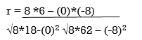
r = 48/√144*√432 = 0.19

Q14) Two variables X and Y are given in the dataset below, find the two lines of regression.

A14)

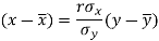
The two lines of regression can be expressed as-

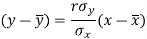
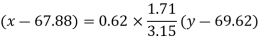
And

x	y			Xy
65	66	4225	4356	4290
66	68	4356	4624	4488
67	65	4489	4225	4355
67	69	4489	4761	4623
68	74	4624	5476	5032
69	73	4761	5329	5037
70	72	4900	5184	5040
71	70	5041	4900	4970
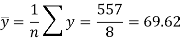
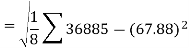
Sum = 543	557	36885	38855	37835

Now-

And

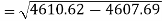
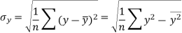
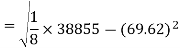
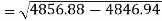
Standard deviation of x-

Similarly-

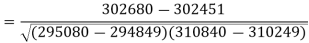
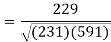
Correlation coefficient-

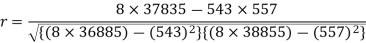
Put these values in regression line equation, we get

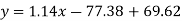
Regression line y on x-

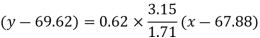
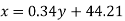
Regression line x on y-

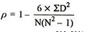
Q15) Compute the Spearman’s rank correlation coefficient of the dataset given below-

A15)

Person	Rank in test-1	Rank in test-2	d =
A	9	1	8	64
B	10	2	8	64
C	6	3	3	9
D	5	4	1	1
E	7	5	2	4
F	2	6	-4	16
G	4	7	-3	9
H	8	8	0	0
I	1	9	-8	64
J	3	10	-7	49
Sum				280

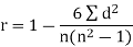
Q16)

A16)

Here, highest value is taken as 1

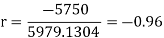
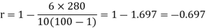
R = 1 – (6*8)/5(52 – 1) = 0.60

Q17) Deduce Lagrange’s formula for interpolation.  The observed values of a function  are respectively  168,120,72 and 63 at the  four position3,7,9 and 10 of  the independent variable. What is the  best estimate you can for  the value of the  function  at the position6 of  the independent variable.

A17)

We construct  the table for the given data:

We need to  calculate for  x =  6, we need f(6)=?

Here

We get

By Lagrange’s interpolation formula,  we have

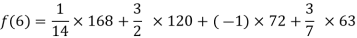
Hence the estimated value for x=6 is 147.

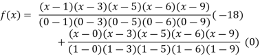
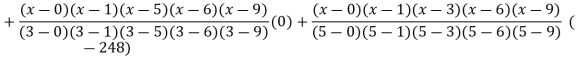
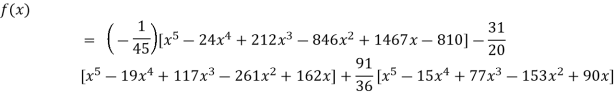
Q18) Find the polynomial of  fifth degree from  the following data

A18)

Here

We get 

By Lagrange’s  interpolation  formula