Unit - 1

Introduction to Algorithm

Q1) What are the Basic Terminologies of Elementary Data Organizations?

A1) Data: Data are simply valuing or set of values

Data Items: It refers to a single unit of values.

Data items are divided into sub-items called Group items.

Ex: Employee Name may be divided into three subitems

First name, Middle name, Last name.

Data items that are not further divided into sub items are called Elementary items.

Entity: An entity is something that has attributes or properties which may be assigned values. The values may be numeric or non-numeric.

Ex: Attributes        Names                 Age         Sex          SSN

Values              Rohland Gail       34              F            134-34-5533

Entities with similar attributes form an entity set. Each attribute of an entity set has a range of values: the set of all possible values that could be assigned to a particular attribute.

Field: is a single elementary unit of information representing an attribute of an entity.

Record: It is a collection of field values of the given entity.

File: is the collection of records of entities in a given entity set.

Each record in a file may contain field items but the value in a certain field may uniquely determine the record in the file. Such a field k is called the primary key and the values k1, k2….kn are called the keys or key values.

Records may also be classified according to length

A file can have fixed-length records or variable length records.

In fixed length records all the records contain the same data items with the same amount of space assigned to each data item.

In variable length records the file records may contain different lengths.

Example:

Student records have variable lengths since different students take different number of courses. Variable length records have a minimum and maximum length

The above organization of data into fields, records and files may not be complex enough to maintain and efficiently process certain collections of data. For this reason, data are also organized into more complex types of structures.

Q2) Define Insertion operation? With an example?

A2) Insert operation is to insert one or more data elements into an array. Based on the requirement, a new element can be added at the beginning, end, or any given index of array.

Here, we see a practical implementation of insertion operation, where we add data at the end of the array −

Example

Following is the implementation of the above algorithm −

#include <stdio.h>

Main() {

Int LA[] = {1,3,5,7,8};

Int item = 10, k = 3, n = 5;

Int i = 0, j = n;

Printf("The original array elements are :\n");

For(i = 0; i<n; i++) {

Printf("LA[%d] = %d \n", i, LA[i]);

}

n = n + 1;

While( j >= k) {

LA[j+1] = LA[j];

j = j - 1;

}

LA[k] = item;

Printf("The array elements after insertion :\n");

For(i = 0; i<n; i++) {

Printf("LA[%d] = %d \n", i, LA[i]);

}

}

When we compile and execute the above program, it produces the following result:

Output

The original array elements are:

LA [0] = 1

LA [1] = 3

LA [2] = 5

LA [3] = 7

LA [4] = 8

The array elements after insertion:

LA [0] = 1

LA [1] = 3

LA [2] = 5

LA [3] = 10

LA [4] = 7

LA [5] = 8

Q3) Define Deletion operation? With an example?

A3) Deletion refers to removing an existing element from the array and re-organizing all elements of an array.

Algorithm

Consider LA is a linear array with N elements and K is a positive integer such that K<=N. Following is the algorithm to delete an element available at the Kth position of LA.

1. Start

2. Set J = K

3. Repeat steps 4 and 5 while J < N

4. Set LA[J] = LA [J + 1]

5. Set J = J+1

6. Set N = N-1

7. Stop

Example

Following is the implementation of the above algorithm −

#include <stdio.h>

Void main() {

Int LA[] = {1,3,5,7,8};

Int k = 3, n = 5;

Int i, j;

Printf("The original array elements are :\n");

For(i = 0; i<n; i++) {

Printf("LA[%d] = %d \n", i, LA[i]);

}

j = k;

While( j < n) {

LA[j-1] = LA[j];

j = j + 1;

}

n = n -1;

Printf("The array elements after deletion :\n");

For(i = 0; i<n; i++) {

Printf("LA[%d] = %d \n", i, LA[i]);

}

}

When we compile and execute the above program, it produces the following result −

Output

The original array elements are:

LA [0] = 1

LA [1] = 3

LA [2] = 5

LA [3] = 7

LA [4] = 8

The array elements after deletion:

LA [0] = 1

LA [1] = 3

LA [2] = 7

LA [3] = 8

Q4) Define Traversal operation? With an example?

A4) Each element of an array is accessed precisely once for processing during an array traversal operation.

This is also known as array visiting.

As an illustration

Let LA be an unordered Linear Array with N item.

/Create a programme to perform a traversal operation.

Void main #include stdio.h> ()

{

Int LA[] = {2,4,6,8,9};

Int i, n = 5;

Printf("The array elements are:\n");

For(i = 0; i < n; i++)

{

Printf("LA[%d] = %d \n", i, LA[i]);

}

}

Output

The original array elements are:

LA [0] = 2

LA [1] = 4

LA [2] = 6

LA [3] = 8

LA [4] = 9

Q5) What is the Analysis of an Algorithm? In brief.

A5) Analysis is the theoretical way to study performance of computer program. Analysis of an algorithm is helpful to decide the complexity of an algorithm.

There are three ways to analyze an algorithm which are stated as below.

1. Worst case: In worst case analysis of an algorithm, upper bound of an algorithm is calculated. This case considers the maximum number of operations on algorithm. For example, if user want to search a word in English dictionary which is not present in the dictionary. In this case user has to check all the words in dictionary for desired word.

2. Best case: In best case analysis of an algorithm, lower bound of an algorithm is calculated. This case considers the minimum number of operations on algorithm. For example, if user want to search a word in English dictionary which is found at the first attempt. In this case there is no need to check other words in dictionary.

3. Average case: In average case analysis of an algorithm, all possible inputs are considered and computing time is calculated for all inputs. Average case analysis is performed by summation of all calculated value which is divided by total number of inputs. In average case analysis user must be aware about the all types of input so average case analysis are very rarely used in practical cases.

Q6) Describe Asymptotic Notations? 

A6) To express the running time complexity of algorithm three asymptotic notations are available. Asymptotic notations are also called as asymptotic bounds. Notations are used to relate the growth of complex functions with the simple function. Asymptotic notations have a domain of natural numbers.

Big-oh notation

Big-oh notations can be expressed by using the ‘o’ symbol. This notation indicates the maximum number of steps required to solve the problem. This notation expresses the worst-case growth of an algorithm. Consider the following diagram in which there are two functions f(x) and g(x). f(x) is more complex than the function g(x).

In the above diagram out of two function f(n) and g(n), more complex function is f(n), so need to relate its growth as compare to simple function g(n). More specifically we need one constant function c(n) which bound function f(n) at some point n0. Beyond the point ‘n0’ function c*g(n) is always greater than f(n).

Now f(n)=Og(n)if there is some constant ‘c’ and some initial value ‘n0’. Such that f(n)<=c*g(n) for all n>n0

In the above expression ‘n’ represents the input size

f(n) represents the time that algorithm will take

f(n) and g(n) are non-negative functions.

Consider the following example

In the above example g(n) is ‘’n’ and f(n) is ‘2n+1’ and value of constant is 3. The point where c*g(n) and f(n) intersect is ‘’n0’. Beyond ‘n0’ c*g(n) is always greater than f(n) for constant ‘3’. We can write the conclusion as follows

f(n)=O g(n) for constant ‘c’ =3 and ‘n0’=1

Such that f(n)<=c*g(n) for all n>n0

Big-omega notation

Big-omega notations can be express by using ‘Ω’ symbol. This notation indicates the minimum number of steps required to solve the problem. This notation expresses the best-case growth of an algorithm. Consider the following diagram in which there are two functions f(n) and g(n). f(n) is more complex than the function g(n).

In the above diagram out of two function f(n) and g(n), more complex function is f(n), so need to relate its growth as compare to simple function g(n). More specifically we need one constant function c(n) which bound function f(n) at some point n0. Beyond the point ‘n0’ function c*g(n) is always smaller than f(n).

Now f(n)=Ωg(n)if there is some constant ‘c’ and some initial value ‘n0’. Such that c*g(n) <= f(n)for all n>n0

In the above expression ‘n’ represents the input size

f(n) represents the time that algorithm will take

f(n) and g(n) are non-negative functions.

Consider the following example

In the above example g(n) is ‘2n’ and f(n) is ‘2n-2’ and value of constant is 0.5. The point where c*g(n) and f(n) intersect is ‘’n0’. Beyond ‘n0’ c*g(n) is always smaller than f(n) for constant ‘0.5’. We can write the conclusion as follows

f(n) = Ω g(n) for constant ‘c’ =0.5 and ‘n0’=2

Such that c*g(n)<= f(n) for all n>n0

Big-theta notation

Big-theta notations can be express by using ‘Ɵ’ symbol. This notation indicates the exact number of steps required to solve the problem. This notation expresses the average case growth of an algorithm. Consider the following diagram in which there are two functions f(n) and g(n). f(n) is more complex than the function g(n).

In the above diagram out of two function f(n) and g(n), more complex function is f(n), so need to relate its growth as compare to simple function g(n). More specifically we need one constant function c1 and c2 which bound function f(n) at some point n0. Beyond the point ‘n0’ function c1*g(n) is always smaller than f(n) and c2*g(n) is always greater than f(n).

Now f(n) = θ g(n) if there is some constant ‘c1 and c2’ and some initial value ‘n0’. Such that c1*g(n) <= f(n)<=c2*g(n)for all n>n0

In the above expression ‘n’ represents the input size

f(n) represents the time that algorithm will take

f(n) and g(n) are non-negative functions.

f(n) = θ g(n) if and only if f(n)=O g(n) and f(n)=Ω g(n)

Consider the following example

In the above example g(n) is ‘2n’ and f(n) is ‘3n-2’ and value of constant c1 is 0.5 and c2 is 2. The point where c*g(n) and f(n) intersect is ‘’n0’. Beyond ‘n0’ c1*g(n) is always smaller than f(n) for constant ‘0.5’ and c2*g(n) is always greater than f(n) for constant ‘2’. We can write the conclusion as follows

f(n)=Ω g(n) for constant ‘c1’ =0.5, ‘c2’ = 2 and ‘n0’=2

Such that c1*g(n)<= f(n)<=c2*g(n) for all n>n0

Q7) What do you mean by Time-Space trade off?

A7) Complexity of an algorithm is the function which gives the running time and space requirement of an algorithm in terms of size of input data. Frequency count refers to the number of times particular instructions executed in a block of code. Frequency count plays an important role in the performance analysis of an algorithm. Each instruction in the algorithm is incremented by one as its execution. Frequency count analysis is the form of priori analysis. Frequency count analysis produces output in terms of time complexity and space complexity.

Q8) Define Time and space complexity?

A8) Time complexity is about to number of times compiler execute basic operations in instruction. That is because basic operations are so defined that the time for the other operations is much less than or at most proportional to the time for the basic operations. To determine time complexity user, need to calculate frequency count and express it in terms of notations. Total time taken by program is the summation of compile time and running time. Out of these two main point to take care about is running time as it depends upon the number and magnitude of input and output.

Space complexity

Space complexity is about the maximum amount of memory required for an algorithm. To determine space complexity users need to calculate frequency count and express it in terms of notations.

Frequency count analysis for this code is as follows

In the above example, for the first four instructions there is no frequency count. For data declaration and the inclusion of header file there is no frequency count. So, for this example has a frequency count for time is 2 and a frequency count for space is 1. So, total frequency count is 3.

Consider the following example

Explanation: In the above example, one is added to frequency count for instruction four and seven after that in fifth instruction is check from zero to five so it will add value six to frequency count. ‘For’ loop executed for five times so for sixth instruction frequency count is five. Total frequency count for above program is 1+6+5+1 =13.

Consider the following example

Explanation: In the above example, in instruction five value of ‘i’ is check from 0 to ‘m’ so frequency count is ‘m+1’ for fifth instruction. In instruction five value of ‘j’ is check from 0 to ‘n’ so frequency count is ‘n+1’ but this instruction is in the for loop which execute for ‘m’ times, so for seventh instruction is m*(n+1). Ninth instruction is in the two for loops, out of which first for loop execute for m times and second ‘for’ loop execute for ‘n’ times. So, for ninth instruction frequency count is m*n. The total frequency count for the above program is (m+1) +m(n+1) +mn=2m+2mn+1=2m(1+n) +1.

Consider the following example

Explanation: For above program total frequency count

=(m+1) +m(n+1) +mn+mn(n+1) +mn

=m+1+mn+m+mn+mn2 +mn+mn2

=2 mn2+3mn+2m+1

=mn(2n+3) +2m+1

Consider the following example

Explanation: the above example, one is added to frequency count for instruction four. The loop will execute till value of n is incremented to 10 from 1, so for loop statements i.e., instructions seven and eight is execute for tem times. When the value of ‘n’ is ten then ‘break’ statement will execute for one time and it will skip the tenth execution of tenth instruction. Tenth instruction will add value nine to frequency count. Total frequency count for above program is 10+10+1+9+10 = 40.

Q9) Define Linear Search Techniques and their complexity analysis?

A9) Thus Algorithm for Linear Search is

1. Start at one end of the list

2. If the current element is not equal to the search target, move to the next element,

3. Stop when a match is found or the opposite end of the list is reached.

Function for Linear search is

Find(values, target)

{

For( i = 0; i < values.length; i++)

{

If (values[i] == target)

{ return i; }

}

Return –1;

}

If an element is found this function returns the index of that element otherwise it returns –1.

Example: we have an array of integers, like the following:

Let’s search for the number 7. According to function for linear search index for element 7 should be returned. We start at the beginning and check the first element in the array.

First element is 9. Match is not found and hence we move to next element i.e., 6.

Again, match is not found so move to next element i.e.,7.

We found the match at the index position 2. Hence output is 2.

If we try to find element 10 in above array, it will return –1, as 10 is not present in the array.

Complexity Analysis of Linear Search:

Let us assume element x is to be searched in array A of size n.

An algorithm can be analyzed using the following three cases.

1. Worst case

2. Average case

3. Best case

1. Worst case: In Linear search worst case happens when element to be searched is not present. When x is not present, the linear search function compares it with all the elements of A one by one. The size of A is n and hence x is to be compared with all n elements. Thus, the worst-case time complexity of linear search would be O(n).

2. Average case: In average case analysis, we take all possible inputs and calculate computing time for all of the inputs. Sum all the calculated values and divide the sum by total number of inputs. Following is the value of average case time complexity.

Average Case Time= ∑=  ×= O (n)

3. Best Case: In linear search, the best case occurs when x is present at the first location. So, time complexity in the best-case would-be O (1).

P1: Program for Linear Search

#include<stdio.h>

#include<conio.h>

Int search(int [],int, int);
void main()
{
 int a[20],k,i,n,m;

Clrscr();

Printf(“\n\n ENTER THE SIZE OF ARRAY”);

Scanf(“%d”,&n);

Printf(“\n\nENTER THE ARRAY ELEMENTS\n\n”);

For(i=0;i<n;i++)
 {
 scanf(“%d”,&a[i]);
 }
 printf(“\n\nENTER THE ELEMENT FOR SEARCH\n”);
 scanf(“%d”,&k);
 m=search(a,n,k);
 if(m==–1)
 {
 printf(“\n\nELEMENT IS NOT FOUND IN LIST”);
 }
 else
 {
 printf(“\n\nELEMENT IS FOUND AT LOCATION %d”,m);
 }
 }
 getch();
 }

Int search(int a[],int n,int k)
 {
 int i;
 for(i=0;i<n;i++)
 {
 if(a[i]==k)
 {
 return i;
 }
 }
 if(i==n)
 {
 return –1;
}

}

Merits:

1. Simple and easy to implement
2. It works well even on unsorted arrays.
3. It is memory efficient as it does not require copying and partitioning of the array being searched.

Demerits:

1. Suitable only for small number of values.
2. It is slow as compared to binary search.

Q10) Define Binary Search Techniques and their complexity analysis?

A10) Binary Search requires a sorted array.

Steps to perform binary search on sorted array A of size n are as follows.

1. Initialize lower and upper limit of array to be searched Low=0, High= n–1.

2. Find the middle position

Mid= (Low + High)/2

3. Compare the input key value with the key value of the middle element of the array. It has 3 possibilities.

Case 1: If keys match then return mid and print element found.

If(key==A[mid])

Return mid

Case 2: If key is less than middle element then element is present in left half of array. Update High and goto step 2. 

If(key<A[mid])

High= Mid–1

Goto step 2

Case 3: If key is greater than middle element then element is present in right half of array. Update Low and goto step 2. 

If(key>A[mid])

Low= Mid+1

Goto step 2

Case 4: if (Low>High)

Print element not found.

Iterative algorithm for Binary Search

Int BinarySearch(int A[],int x)

{

Int mid,n;

Int Low = 0;

Int High = n–1;

While ( Low <= High )

{

Mid = (Low + High) / 2;

If ( A[mid] == x )

Return mid;

If ( A[mid] > x )

High = mid – 1;

Else Low = mid + 1;

}

Return –1;

}

Q11) Explain selection algorithms?

A11) Assume we want to sort the list in ascending order. Selection sort finds the smallest element from an unsorted list and swap it with the element in first position. Then it finds the second smallest element and swaps it with the element at second position. This process is repeated till the entire list is sorted in ascending order. Each time we swap elements, we say that we have completed a sort pass. A list of n elements requires n–1 passes to completely rearrange the data.

Procedure for every pass is as follows.

Pass 1: Find the position P of the smallest in the list of N elements A[l], A [2], . . ., A[N], and then interchange A[P] and A [1]. Then A [1] is sorted.

Pass 2: Find the position P of the smallest in the sublist of N –1 element A [2], A [3], . . ., A[N], and then interchange A[P]and A [2]. Then A[l], A [2] is sorted.

Pass 3: Find the position P of the smallest in the sublist of N–2 elements A [3], A [4], . . ., A[N], and then interchange A[P] and A [3]. Then: A[l], A [2], A [3] is sorted.

Pass N –1: Find the position P of the smaller of the elements A [N –1), A[N], and then interchange A[P] and A[N–1]. Then: A[l], A [2], . . ., A[N] is sorted. Thus, A is sorted after N –1 passes.

Example 1:      

Fig.: Original List

We will apply selection sort on this list.

Pass 1:

Here smallest element is 9 and 25 is located at first position. So, we swap 9 with 25.

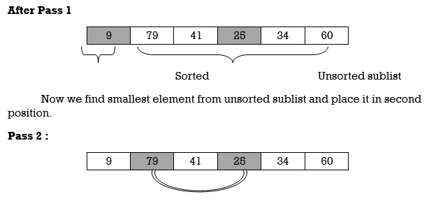
Unsorted sublist has 25 as a smallest element and 79 is located at second position. Hence, we swap 25 and 79.

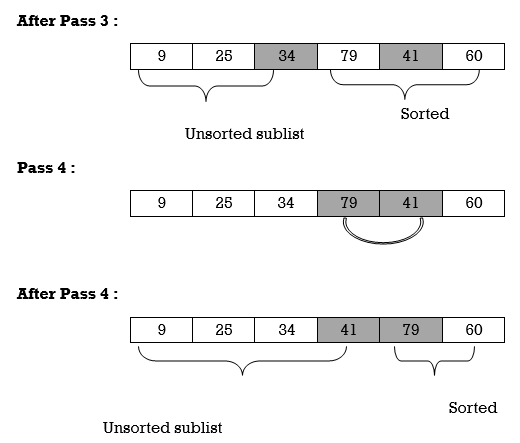
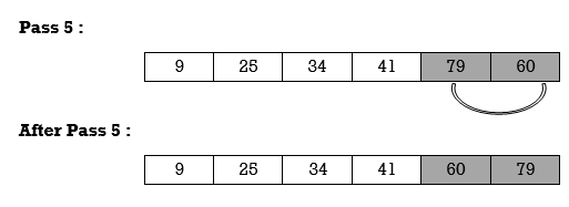
Thus, list is sorted.

We will see one more example.

Apply selection sort on array A= {77,30,40,10,88,20,65,56}

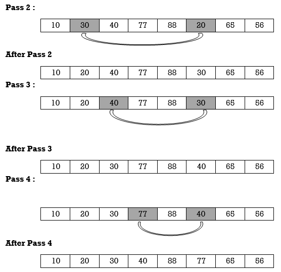
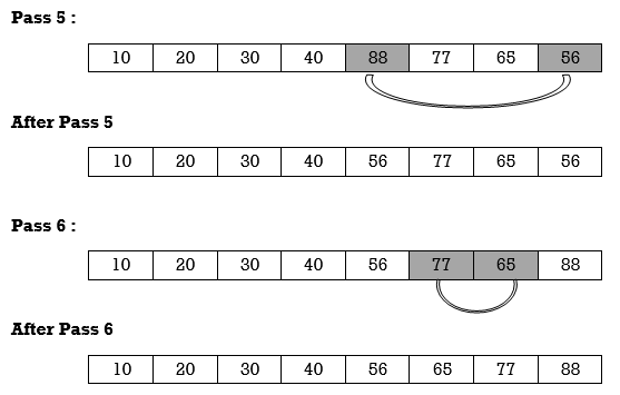
Hence the list is sorted in ascending order by applying selection sort.

Function for Selection Sort

Void selectionSort(int A[], int n)

{

Int i, j, s, temp;

For (i= 0; i <= n; i ++)

{

s = i;

For (j=i+1; j <= n; j++)

If(A[j] < A[s])

s= j;

// Smallest selected; swap with current element

Temp = A[i];

A[i] = A[s];

A[s] = temp;

}

P4: Program to perform Selection Sort.

#include <stdio.h>

Int main()

{

Int A[100], n, i, j, s, temp;

/* n=total no. Of elements in array

s= smallest element in unsorted array

Temp is used for swapping */

Printf("Enter number of elements\n");

Scanf("%d", &n);

Printf("Enter %d integers\n", n);

For ( i = 0 ; i < n ; i++ )

Scanf("%d", &A[i]);

For ( i = 0 ; i < ( n – 1 ) ; i++ )

{

s = i;

For ( j = i + 1 ; j < n ; j++ )

{

If ( A[s] > A[j] )

s = j;

}

If ( s != i )

{

Temp = A[i];

A[i] = A[s];

A[s] = temp;

}

}

Printf("Sorted list in ascending order:\n");

For ( i = 0 ; i < n ; i++ )

Printf("%d\n", A[i]);

Return 0;

}

Output:

Enter number of elements

5

Enter 5 integers

4

1

7

5

9

Sorted list in ascending order

1

4

5

7

9

Q12) What are the Complexity of Selection Sort?

A12) In selection sort outer for loop is executed n–1 time. On the kth time through the

Outer loop, initially the sorted list holds

k–1 elements and unsorted portion holds n–k+1 elements. In inner for loop 2

Elements are compared each time.

Thus, 2*(n–k) elements are examined by the inner loop during the kth pass through

The outer loop. But k ranges from 1 to n–1.

Total number of elements examined is:

T(n) = 2*(n –1) + 2*(n–2) + 2*(n–3) + ... + 2*(n–(n–2)) + 2*(n–(n–1))

=2*((n–1) + (n–2) + (n–3) + ... + 2 + 1)

(Or 2*(sum of first n–1 integers)

=2*((n–1) *n)/2)

=n 2 – n, so complexity of algorithm is O(n 2 ).

Q13) Define Insertion Sort with example?

A13) Insertion Sort reads all elements from 1 to n and inserts each element at its proper position. This sorting method works well on small list of elements. 

Procedure for each pass is as follows.

Pass 1:

A[l] by itself is trivially sorted.

Pass 2:

A [2] is inserted either before or after A[l] so that: A[l], A [2] is sorted.

Pass 3:

A [3] is inserted into its proper place so that: A[l], A [2], A [3] is sorted.

Pass 4:

A [4] is inserted into its proper place A[l], A [2], A [3], A [4] is sorted.

Pass N: A[N] is inserted into its proper place in so that: A[l], A [ 2], . . ., A [ N] is sorted

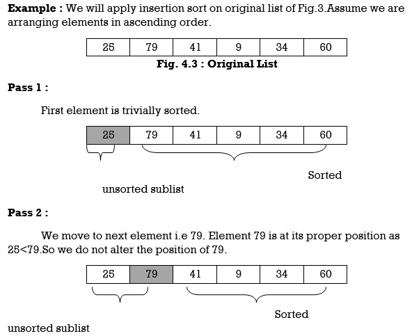
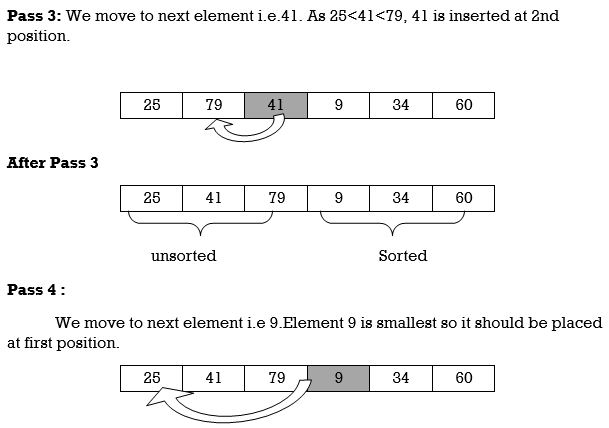
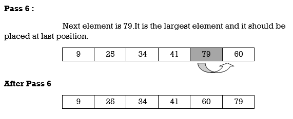
Hence the list is sorted using insertion sort.

We will see one more example.

Apply Insertion sort on array A= {77,30,40,10,88,20,65,56}

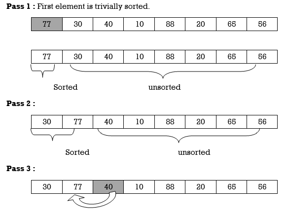
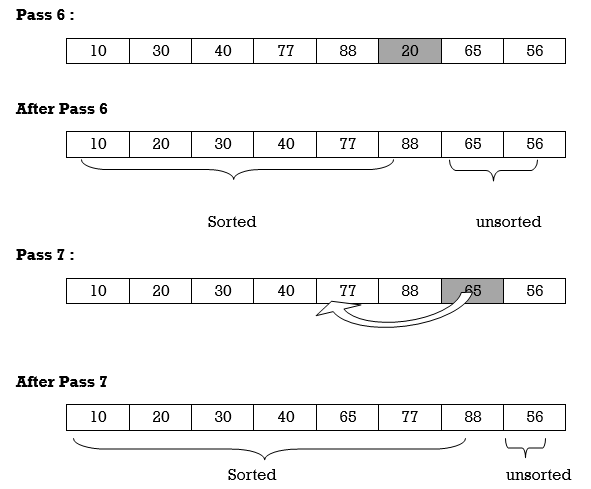
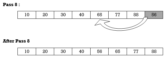
Hence the list is sorted using Insertion sort.

C Function for Insertion Sort

Void insertionSort(int A[], int n)

{

Int i, p, temp, j;

For (i = 1; i<=n; i++)

{

p= 0;

Temp = A[i];

For (j=i–1; j >= 0 && !p;)

If(temp < A[j])

{

A[j + 1]= A[j];

j––;

}

Else

p = 1;

A[j + 1] = temp;

}

Return;

}

P5: Program to implement insertion sort.

#include <stdio.h>

Int main()

{

Int n, A[100], i, j, t;

Printf("Enter number of elements\n");

Scanf("%d", &n);

Printf("Enter %d integers\n", n);

For (i = 0; i < n; i++) {

Scanf("%d", &A[i]);

}

For (i = 1 ; i <=( n – 1); i++)

{

j = i;

While ( j > 0 && A[j] < A[j–1])

{

t  = A[j];

A[j]   = A[j–1];

A[j–1] = t;

j––;

}

}

Printf("Sorted list in ascending order:\n");

For (i = 0; i <= n – 1; i++) {

Printf("%d\n", A[i]);

}

Return 0;

}

Output:

Enter number of elements

5

Enter 5 integers

9

4

2

5

3

Sorted list in ascending order

2

3

4

5

9

Q14) What is Heap Sort with an example?

A14) Heap is a special tree-based data structure. A binary tree is said to follow a heap data structure if it is a complete binary tree.

All nodes in the tree follow the property that they are greater than their children i.e., the largest element is at the root and both its children and smaller than the root and so on. Such a heap is called a max-heap. If instead, all nodes are smaller than their children, it is called a min-heap.

The following example diagram shows Max-Heap and Min-Heap.

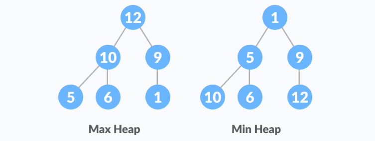
Starting from a complete binary tree, we can modify it to become a Max-Heap by running a function called heapify on all the non-leaf elements of the heap.

Heapify(array)

Root = array [0]

Largest = largest (array [0], array [2*0 + 1]. Array [2*0+2])

If (Root! = Largest)

Swap (Root, Largest)

The example above shows two scenarios - one in which the root is the largest element and we don't need to do anything. And another in which the root had a larger element as a child and we needed to swap to maintain max-heap property

Q15) Explain in place / outplace technique?

A15) A sorting technique is in place if it does not use any extra memory to sort the array.

Among the comparison-based techniques discussed, only merge sort is outplaced technique as it requires an extra array to merge the sorted subarrays.

Among the non-comparison-based techniques discussed, all are outplaced techniques. Counting sort uses a counting array and bucket sort uses a hash table for sorting the array.

Q16) Explain online / offline technique?

A16) A sorting technique is considered Online if it can accept new data while the procedure is ongoing i.e., complete data is not required to start the sorting operation.

Among the comparison-based techniques discussed, only Insertion Sort qualifies for this because of the underlying algorithm it uses i.e., it processes the array (not just elements) from left to right and if new elements are added to the right, it doesn’t impact the ongoing operation.

Q17) Explain stable/ unstable technique?

A17) A sorting technique is stable if it does not change the order of elements with the same value.

Out of comparison-based techniques, bubble sort, insertion sort and merge sort are stable techniques. Selection sort is unstable as it may change the order of elements with the same value. For example, consider the array 4, 4, 1, 3.

In the first iteration, the minimum element found is 1 and it is swapped with 4 at 0th position. Therefore, the order of 4 with respect to 4 at the 1st position will change. Similarly, quick sort and heap sort are also unstable.

Q18) Write the difference between linear and binary search?

A18) Difference between Linear and Binary search

Q19) Write any example of binary search?

A19) Let us consider an array arr = {1, 5, 7, 8, 13, 19, 20, 23, 29}. Find the location of the item 23 in the array.

In 1st step:

1. BEG = 0  
2. END = 8ron 
3. MID = 4  
4. a[mid] = a[4] = 13 < 23, therefore 

In Second step:

1. Beg = mid +1 = 5  
2. End = 8 
3. Mid = 13/2 = 6   
4. a[mid] = a[6] = 20 < 23, therefore;  

In third step:

1. Beg = mid + 1 = 7  
2. End = 8  
3. Mid = 15/2 = 7 
4. a[mid] = a[7]  
5. a[7] = 23 = item;  
6. Therefore, set location = mid;  
7. The location of the item will be 7. 

Q20) What do you mean by best, average and worst analysis?

A20) We all know that as the input size (n) grows, the running time of an algorithm grows (or stays constant in the case of constant running time). Even if the input has the same size, the running duration differs between distinct instances of the input. In this situation, we examine the best, average, and worst-case scenarios. The best case running time is the shortest, the worst case running time is the longest, and the average case running time is the time required to execute the algorithm on average. All of these principles will be explained using two examples: I linear search and (ii) insertion sort.

Best case

Consider the case of Linear Search, in which we look for a certain item in an array. We return the relevant index if the item is in the array; else, we return -1. The linear search code is provided below.

Int search(int a, int n, int item) {

Int i;

For (i = 0; i < n; i++) {

If (a[i] == item) {

Return a[i]

}

}

Return -1

}

Variable an is an array, n is the array's size, and item is the array item we're looking for. It will return the index immediately if the item we're seeking for is in the very first position of the array. The for loop is just executed once. In this scenario, the complexity will be O. (1). This is referred to be the best case scenario.

Average case

On occasion, we perform an average case analysis on algorithms. The average case is nearly as severe as the worst scenario most of the time. When attempting to insert a new item into its proper location using insertion sort, we compare the new item to half of the sorted items on average. The complexity remains on the order of n2, which corresponds to the worst-case running time.

Analyzing an algorithm's average behavior is usually more difficult than analyzing its worst-case behavior. This is due to the fact that it is not always clear what defines a "average" input for a given situation. As a result, a useful examination of an algorithm's average behavior necessitates previous knowledge of the distribution of input instances, which is an impossible condition. As a result, we frequently make the assumption that all inputs of a given size are equally likely and do the probabilistic analysis for the average case.

Worst case

In real life, we almost always perform a worst-case analysis on an algorithm. The longest running time for any input of size n is called the worst case running time.

The worst case scenario in a linear search is when the item we're looking for is at the last place of the array or isn't in the array at all. We must run through all n elements in the array in both circumstances. As a result, the worst-case runtime is O. (n). In the case of linear search, worst-case performance is more essential than best-case performance for the following reasons.

●      Rarely is the object we're looking for in the first position. If there are 1000 entries in the array, start at 1 and work your way up. There is a 0.001% probability that the item will be in the first place if we search it at random from 1 to 1000.

●      Typically, the item isn't in the array (or database in general). In that situation, the worst-case running time is used.

Similarly, when items are reverse sorted in insertion sort, the worst case scenario occurs. In the worst scenario, the number of comparisons will be on the order of n2, and hence the running time will be O (n2).

Knowing an algorithm's worst-case performance ensures that the algorithm will never take any longer than it does today.