Unit - 5

Graphs and Hashing

Q1) What is Basic Terminology and Representation of the Graph?

A1) Graph is a non-linear data structure. It contains a set of points known as nodes (or vertices) and a set of links known as edges (or Arcs). Here edges are used to connect the vertices. A graph is defined as follows…

Graph is a collection of vertices and arcs in which vertices are connected with arcs Graph is a collection of nodes and edges in which nodes are connected with edges

Generally, a graph G is represented as G = (V, E), where V is set of

Vertices and E is set of edges.

Example

The following is a graph with 5 vertices and 6 edges.

This graph G can be defined as G = (V, E)

Where V = {A, B, C, D, E} and E = {(A, B), (A, C) (A, D), (B, D), (C, D), (B, E), (E, D)}.

Graph Terminology

We use the following terms in graph data structure…

Vertex

Individual data element of a graph is called as Vertex. Vertex is also known as node. In above example graph, A, B, C, D & E are known as vertices.

Edge

An edge is a connecting link between two vertices. Edge is also known as Arc. An edge is represented as (startingVertex, endingVertex). For example, in above graph the link between vertices A and B is represented as (A, B). In above example graph, there are 7 edges (i.e., (A, B), (A, C), (A, D), (B, D), (B, E), (C, D), (D, E)).

Edges are three types.

1. Undirected Edge - An undirected edge is a bidirectional edge. If there is undirected edge between vertices A and B then edge (A, B) is equal to edge (B, A).
2. Directed Edge - A directed edge is a unidirectional edge. If there is directed edge between vertices A and B then edge (A, B) is not equal to edge (B, A).
3. Weighted Edge - A weighted edge is an edge with value (cost) on it.

Undirected Graph

A graph with only undirected edges is said to be undirected graph.

Directed Graph

A graph with only directed edges is said to be directed graph.

Mixed Graph

A graph with both undirected and directed edges is said to be mixed graph.

End vertices or Endpoints

The two vertices joined by edge are called end vertices (or endpoints) of that edge.

Origin

If an edge is directed, its first endpoint is said to be the origin of it.

Destination

If an edge is directed, its first endpoint is said to be the origin of it and the other endpoint is said to be the destination of that edge.

Adjacent

If there is an edge between vertices A and B then both A and B are said to be adjacent. In other words, vertices A and B are said to be adjacent if there is an edge between them.

Incident

Edge is said to be incident on a vertex if the vertex is one of the endpoints of that edge.

Outgoing Edge

A directed edge is said to be outgoing edge on its origin vertex.

Incoming Edge

A directed edge is said to be incoming edge on its destination vertex.

Degree

Total number of edges connected to a vertex is said to be degree of that vertex.

Indegree

Total number of incoming edges connected to a vertex is said to be indegree of that vertex.

Outdegree

Total number of outgoing edges connected to a vertex is said to be outdegree of that vertex.

Parallel edges or Multiple edges

If there are two undirected edges with same end vertices and two directed edges with same origin and destination, such edges are called parallel edges or multiple edges.

Self-loop

Edge (undirected or directed) is a self-loop if its two endpoints coincide with each other.

Simple Graph

A graph is said to be simple if there are no parallel and self-loop edges.

Path

A path is a sequence of alternate vertices and edges that starts at a vertex and ends at other vertex such that each edge is incident to its predecessor and successor vertex.

Q2) Define Graph Search and its Traversal algorithms?

A2) Depth First Traversal (or Search) for a graph is similar to Depth First Traversal of a tree. The only catch here is, unlike trees, graphs may contain cycles, a node may be visited twice. To avoid processing a node more than once, use a Boolean visited array.

Example:

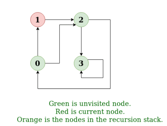
Input: n = 4, e = 6

0 -> 1, 0 -> 2, 1 -> 2, 2 -> 0, 2 -> 3, 3 -> 3

Output: DFS from vertex 1: 1 2 0 3

Explanation:

DFS Diagram:

Input: n = 4, e = 6

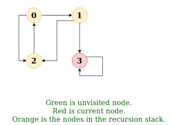
2 -> 0, 0 -> 2, 1 -> 2, 0 -> 1, 3 -> 3, 1 -> 3

Output: DFS from vertex 2: 2 0 1 3

Explanation:

DFS Diagram:

Q3) Define Hashing?

A3) Hashing is an important Data Structure which is designed to use a special function called the Hash function which is used to map a given value with a particular key for faster access of elements. The efficiency of mapping depends of the efficiency of the hash function used.

Let a hash function H(x) maps the value  at the index x%10 in an Array. For example, if the list of values is [11,12,13,14,15] it will be stored at positions {1,2,3,4,5} in the array or Hash table respectively.

Q4) Explain Hashing?

A4) Hashing is a technique to convert a range of key values into a range of indexes of an array. We're going to use modulo operator to get a range of key values. Consider an example of hash table of size 20, and the following items are to be stored. Item are in the (key,value) format.

●        (1,20)

●        (2,70)

●        (42,80)

●        (4,25)

●        (12,44)

●        (14,32)

●        (17,11)

●        (13,78)

●        (37,98)

Q5) What is Linear Probing?

A5) As we can see, it may happen that the hashing technique is used to create an already used index of the array. In such a case, we can search the next empty location in the array by looking into the next cell until we find an empty cell. This technique is called linear probing.

Q6) Explain Search Operation of hash table?

A6) Whenever an element is to be searched, compute the hash code of the key passed and locate the element using that hash code as index in the array. Use linear probing to get the element ahead if the element is not found at the computed hash code.

Example

Struct DataItem *search(int key) {

//get the hash

Int hashIndex = hashCode(key);

//move in array until an empty

While(hashArray[hashIndex] != NULL) {

If(hashArray[hashIndex]->key == key)

Return hashArray[hashIndex];

//go to next cell

++hashIndex;

//wrap around the table

HashIndex %= SIZE;

}

Return NULL;       

}

Q7) Explain Insert Operation of hash table?

A7) Whenever an element is to be inserted, compute the hash code of the key passed and locate the index using that hash code as an index in the array. Use linear probing for empty location, if an element is found at the computed hash code.

Example

Void insert(int key,int data) {

Struct DataItem *item = (struct DataItem*) malloc(sizeof(struct DataItem));

Item->data = data; 

Item->key = key;    

//get the hash

Int hashIndex = hashCode(key);

//move in array until an empty or deleted cell

While(hashArray[hashIndex] != NULL && hashArray[hashIndex]->key != -1) {

//go to next cell

++hashIndex;

//wrap around the table

HashIndex %= SIZE;

}

HashArray[hashIndex] = item;       

}

Q8) Explain Delete Operation of hash table?

A8) Whenever an element is to be deleted, compute the hash code of the key passed and locate the index using that hash code as an index in the array. Use linear probing to get the element ahead if an element is not found at the computed hash code. When found, store a dummy item there to keep the performance of the hash table intact.

Example

Struct DataItem* delete(struct DataItem* item) {

Int key = item->key;

//get the hash

Int hashIndex = hashCode(key);

//move in array until an empty

While(hashArray[hashIndex] !=NULL) {

If(hashArray[hashIndex]->key == key) {

Struct DataItem* temp = hashArray[hashIndex];

//assign a dummy item at deleted position

HashArray[hashIndex] = dummyItem;

Return temp;

}

//go to next cell

++hashIndex;

//wrap around the table

HashIndex %= SIZE;

} 

Return NULL;       

}

Hash Table is a data structure which stores data in an associative manner. In hash table, the data is stored in an array format where each data value has its own unique index value. Access of data becomes very fast, if we know the index of the desired data.

Q9) Explain Searching Techniques of hash table?

A9) In data structures,

●        There are several searching techniques like linear search, binary search, search trees etc.

●        In these techniques, time taken to search any particular element depends on the total number of elements.

Example-

●        Linear search takes O(n) time to perform the search in unsorted arrays consisting of n elements.

●        Binary Search takes O(logn) time to perform the search in sorted arrays consisting of n elements.

●        It takes O(logn) time to perform the search in BST consisting of n elements.

Drawback-

The main drawback of these techniques is-

●        As the number of elements increases, time taken to perform the search also increases.

●        This becomes problematic when total number of elements become too large.

Hashing in Data Structure-

In data structures,

●        Hashing is a well-known technique to search any particular element among several elements.

●        It minimizes the number of comparisons while performing the search.

Advantage-

Unlike other searching techniques,

●        Hashing is extremely efficient.

●        The time taken by it to perform the search does not depend upon the total number of elements.

●        It completes the search with constant time complexity O(1).

Q10) What are the Types of Hash Functions?

A10) There are various types of hash functions available such as-

1. Mid Square Hash Function
2. Division Hash Function
3. Folding Hash Function etc

It depends on the user which hash function he wants to use.

Properties of Hash Function-

The properties of a good hash function are-

●        It is efficiently computable.

●        It minimizes the number of collisions.

●        It distributes the keys uniformly over the table.

Q11) What are the Characteristics of Good Hash Function?

A11) Characteristics of good Hash Function

1. The hash value is fully determined by the data being hashed.
2. The hash Function uses all the input data.
3. The hash function "uniformly" distributes the data across the entire set of possible hash values.
4. The hash function generates complicated hash values for similar strings.

Some Popular Hash Function is:

1. Division Method:

Choose a number m smaller than the number of n of keys in k (The number m is usually chosen to be a prime number or a number without small divisors, since this frequently a minimum number of collisions).

The hash function is:

For Example: if the hash table has size m = 12 and the key is k = 100, then h (k) = 4. Since it requires only a single division operation, hashing by division is quite fast.

2. Multiplication Method:

The multiplication method for creating hash functions operates in two steps. First, we multiply the key k by a constant A in the range 0 < A < 1 and extract the fractional part of kA. Then, we increase this value by m and take the floor of the result.

The hash function is:

Where "k A mod 1" means the fractional part of k A, that is, k A -⌊k A⌋.

3. Mid Square Method:

The key k is squared. Then function H is defined by

H (k) = L  

Where L is obtained by deleting digits from both ends of k2. We emphasize that the same position of k2 must be used for all of the keys.

4. Folding Method:

The key k is partitioned into a number of parts k1, k2.... kn where each part except possibly the last, has the same number of digits as the required address.

Then the parts are added together, ignoring the last carry.

H (k) = k1+ k2+.....+kn

Example: Company has 68 employees, and each is assigned a unique four- digit employee number. Suppose L consist of 2- digit addresses: 00, 01, and 02....99. We apply the above hash functions to each of the following employee numbers:

1. 3205,       7148,       2345  

(a) Division Method: Choose a Prime number m close to 99, such as m =97, Then

1. H (3205) = 4,       H (7148) = 67,          H (2345) = 17.  

That is dividing 3205 by 17 gives a remainder of 4, dividing 7148 by 97 gives a remainder of 67, dividing 2345 by 97 gives a remainder of 17.

(b) Mid-Square Method:

k = 3205       7148       2345

k2= 10272025   51093904   5499025

h (k) = 72     93         99

Observe that fourth & fifth digits, counting from right are chosen for hash address.

(c) Folding Method: Divide the key k into 2 parts and adding yields the following hash address:

1. H (3205) = 32 + 50 = 82     H (7148) = 71 + 84 = 55  
2. H (2345) = 23 + 45 = 68  

Q12) Why do we need Hashing?

A12) Suppose we have 50 employees, and we have to give 4 digit key to each employee (as for security), and we want after entering a key, direct user map to a particular position where data is stored.

If we give the location number according to 4 digits, we will have to reserve 0000 to 9999 addresses because anybody can use anyone as a key. There is a lot of wastage.

In order to solve this problem, we use hashing which will produce a smaller value of the index of the hash table corresponding to the key of the user.

Universal Hashing

Let H be a finite collection of hash functions that map a given universe U of keys into the range {0, 1..... m-1}. Such a collection is said to be universal if for each pair of distinct keys k,l∈U, the number of hash functions h∈ H for which h(k)= h(l) is at most |H|/m. In other words, with a hash function randomly chosen from H, the chance of a collision between distinct keys k and l is no more than the chance 1/m of a collision if h(k) and h(l)were randomly and independently chosen from the set {0,1,...m-1}.

Rehashing

If any stage the hash table becomes nearly full, the running time for the operations of will start taking too much time, insert operation may fail in such situation, the best possible solution is as follows:

1. Create a new hash table double in size.
2. Scan the original hash table, compute new hash value and insert into the new hash table.
3. Free the memory occupied by the original hash table.

Q13) Using the hash function ‘key mod 7’, insert the following sequence of keys in the hash table- 50, 700, 76, 85, 92, 73 and 101Use separate chaining technique for collision resolution?

A13) The given sequence of keys will be inserted in the hash table as-

Step-01:

●        Draw an empty hash table.

●        For the given hash function, the possible range of hash values is [0, 6].

●        So, draw an empty hash table consisting of 7 buckets as-

Step-02:

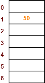
●        Insert the given keys in the hash table one by one.

●        The first key to be inserted in the hash table = 50.

●        Bucket of the hash table to which key 50 maps = 50 mod 7 = 1.

●        So, key 50 will be inserted in bucket-1 of the hash table as-

Step-03 

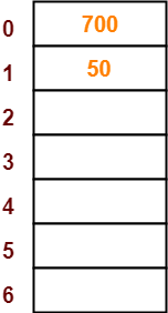
●        The next key to be inserted in the hash table = 700.

●        Bucket of the hash table to which key 700 maps = 700 mod 7 = 0.

●        So, key 700 will be inserted in bucket-0 of the hash table as-

Step-04:

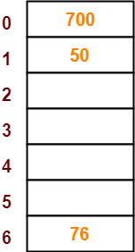
●        The next key to be inserted in the hash table = 76.

●        Bucket of the hash table to which key 76 maps = 76 mod 7 = 6.

●        So, key 76 will be inserted in bucket-6 of the hash table as-

Step-05:

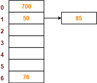
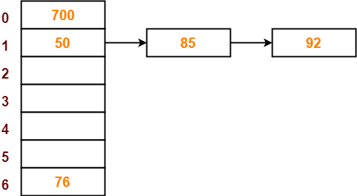
●        The next key to be inserted in the hash table = 85.

●        Bucket of the hash table to which key 85 maps = 85 mod 7 = 1.

●        Since bucket-1 is already occupied, so collision occurs.

●        Separate chaining handles the collision by creating a linked list to bucket-1.

●        So, key 85 will be inserted in bucket-1 of the hash table as-

Step-06:

●        The next key to be inserted in the hash table = 92.

●        Bucket of the hash table to which key 92 maps = 92 mod 7 = 1.

●        Since bucket-1 is already occupied, so collision occurs.

●        Separate chaining handles the collision by creating a linked list to bucket-1.

●        So, key 92 will be inserted in bucket-1 of the hash table as-

Step-07:

●        The next key to be inserted in the hash table = 73.

●        Bucket of the hash table to which key 73 maps = 73 mod 7 = 3.

●        So, key 73 will be inserted in bucket-3 of the hash table as-

Step-08:

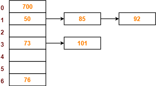
●        The next key to be inserted in the hash table = 101.

●        Bucket of the hash table to which key 101 maps = 101 mod 7 = 3.

●        Since bucket-3 is already occupied, so collision occurs.

●        Separate chaining handles the collision by creating a linked list to bucket-3.

●        So, key 101 will be inserted in bucket-3 of the hash table as-

Q14) Explain depth first search?

A13) Depth First Search is an algorithm for traversing or searching a graph.

It starts from some node as the root node and explores each and every branch of that node before backtracking to the parent node.

DFS is an uninformed search that progresses by expanding the first child node of the graph that appears and thus going deeper and deeper until a goal node is found, or until it hits a node that has no children.

Then the search backtracks, returning to the most recent node it hadn't finished exploring. In a non-recursive implementation, all freshly expanded nodes are added to a LIFO stack for expansion.

Steps for implementing Depth first search

Step 1: - Define an array A or Vertex that store Boolean values, its size should be greater or equal to the number of vertices in the graph G.

Step 2: - Initialize the array A to false

Step 3: - For all vertices v in G

If A[v] = false

Process (v)

Step 4: - Exit

Algorithm for DFS

DFS(G)

{

For each v in V, //for loop V+1 times

{

Color[v]=white; // V times

p[v]=NULL; // V times

}

Time=0; // constant time O (1)

For each u in V, //for loop V+1 times

If (color[u]==white) // V times

DFSVISIT(u) // call to DFSVISIT(v), at most V times O(V)

}

DFSVISIT(u)

{

Color[u]=gray; // constant time

t[u] = ++time;

For each v in Adj(u) // for loop

If (color[v] == white)

{

p[v] = u;

DFSVISIT(v); // call to DFSVISIT(v)

}

Color[u] = black; // constant time

f[u]=++time; // constant time

}

DFS algorithm used to solve following problems:

●      Testing whether graph is connected.

●      Computing a spanning forest of graph.

●      Computing a path between two vertices of graph or equivalently reporting that no such path exists.

●      Computing a cycle in graph or equivalently reporting that no such cycle exists.

Analysis of DFS

In the above algorithm, there is only one DFSVISIT(u) call for each vertex u in the vertex set V. Initialization complexity in DFS(G) for loop is O(V). In second for loop of DFS(G), complexity is O(V) if we leave the call of DFSVISIT(u).

Now, let us find the complexity of function DFSVISIT(u)

The complexity of for loop will be O(deg(u)+1) if we do not consider the recursive call to DFSVISIT(v). For recursive call to DFSVISIT(v), (complexity will be O(E) as

Recursive call to DFSVISIT(v) will be at most the sum of degree of adjacency for all vertex v in the vertex set V. It can be written as ∑ |Adj(v)|=O(E) vεV

The running time of DSF is (V + E).

Q15) Describe Breadth first search?

A14) It is an uninformed search methodology which first expand and examine all nodes of graph systematically in search of the solution in the sequence and then go at the deeper level. In other words, it exhaustively searches the entire graph without considering the goal until it finds it.

From the standpoint of the algorithm, all child nodes obtained by expanding a node are added to a FIFO queue. In typical implementations, nodes that have not yet been examined for their neighbors are placed in some container (such as a queue or linked list) called "open" and then once examined are placed in the container "closed".

Steps for implementing Breadth first search

Step 1: - Initialize all the vertices by setting Flag = 1

Step 2: - Put the starting vertex A in Q and change its status to the waiting state by setting Flag = 0

Step 3: - Repeat through step 5 while Q is not NULL

Step 4: - Remove the front vertex v of Q. Process v and set the status of v to the processed status by setting Flag = -1

Step 5: - Add to the rear of Q all the neighbour of v that are in the ready state by setting Flag = 1 and change their status to the waiting state by setting flag = 0

Step 6: - Exit

Algorithm for BFS

BFS (G, s)

{

For each v in V - {s} // for loop {

Color[v]=white;

d[v]= INFINITY;

p[v]=NULL;

}

Color[s] = gray;

d[s]=0;

p[s]=NULL;

Q = ø; // Initialize queue is empty

Enqueue(Q, s); /* Insert start vertex s in Queue Q */

While Q is nonempty // while loop

{

u = Dequeue[Q]; /* Remove an element from Queue Q*/

For each v in Adj[u] // for loop

{  if (color[v]  == white) /*if v is unvisted*/

{

Color[v] = gray; /* v is visted */

d[v] = d[u] + 1; /*Set distance of v to no. Of edges from s to u*/

p[v] = u;  /*Set parent of v*/

Enqueue(Q,v); /*Insert  v in Queue Q*/

}

}

Color[u] = black; /*finally visted or explored vertex u*/

}

}

Breadth First Search algorithm used in

●      Prim's MST algorithm.

●      Dijkstra's single source shortest path algorithm.

●      Testing whether graph is connected.

●      Computing a cycle in graph or reporting that no such cycle exists.

Analysis of BFS

In this algorithm first for loop executes at most O(V) times.

While loop executes at most O(V) times as every vertex v in V is enqueued only once in the Queue Q. Every vertex is enqueued once and dequeued once so queuing will take at most O(V) time.

Inside while loop, there is for loop which will execute at most O(E) times as it will be at most the sum of degree of adjacency for all vertex v in the vertex set V.

Which can be written as

∑ |Adj(v)|=O(E)

vεV

Total running time of BFS is O(V + E).

Like depth first search, BFS traverse a connected component of a given graph and defines a spanning tree.

Space complexity of DFS is much lower than BFS (breadth-first search). It also lends itself much better to heuristic methods of choosing a likely-looking branch. Time complexity of both algorithms are proportional to the number of vertices plus the number of edges in the graphs they traverse.

Q16) Compare DFS and BFS?

A15) Difference between DFS and BFS