Unit - 2

Relational Data Model

Q1) Explain in brief relational data model?

A1) Relational data model is the primary data model, which is used widely around the world for data storage and processing. This model is simple and it has all the properties and capabilities required to process data with storage efficiency.

Concepts

Tables−In relational data model, relations are saved in the format of Tables. This format stores the relation among entities. A table has rows and columns, where rows represents records and columns represent the attributes.

Tuple− A single row of a table, which contains a single record for that relation is called a tuple.

Relation instance− A finite set of tuples in the relational database system represents relation instance. Relation instances do not have duplicate tuples.

Relation schema− A relation schema describes the relation name (table name), attributes, and their names.

Relation key−Each row has one or more attributes, known as relation key, which can identify the row in the relation (table) uniquely.

Attribute domain−Every attribute has some predefined value scope, known as attribute domain.

Constraints

Every relation has some conditions that must hold for it to be a valid relation. These conditions are called Relational Integrity Constraints. There are three main integrity constraints −

●        Key constraints

●        Domain constraints

●        Referential integrity constraints

Key Constraints

There must be at least one minimal subset of attributes in the relation, which can identify a tuple uniquely. This minimal subset of attributes is called key for that relation. If there are more than one such minimal subsets, these are called candidate keys.

Key constraints force that −

• In a relation with a key attribute, no two tuples can have identical values for key attributes.
• A key attribute cannot have NULL values
• Key constraints are also referred to as Entity Constraints.

Domain Constraints

Attributes have specific values in real-world scenario. For example, age can only be a positive integer. The same constraints have been tried to employ on the attributes of a relation. Every attribute is bound to have a specific range of values. For example, age cannot be less than zero and telephone numbers cannot contain a digit outside 0-9.

Referential integrity Constraints

Referential integrity constraints work on the concept of Foreign Keys. A foreign key is a key attribute of a relation that can be referred in other relation.

Referential integrity constraint states that if a relation refers to a key attribute of a different or same relation, then that key element must exist.

Q2) Write short notes on database schema and database instance?

A2) Database Schema

A database schema is the skeleton structure that represents the logical view of the entire database. It defines how the data is organized and how the relations among them are associated. It formulates all the constraints that are to be applied on the data.

A database schema defines its entities and the relationship among them. It contains a descriptive detail of the database, which can be depicted by means of schema diagrams. It’s the database designers who design the schema to help programmers understand the database and make it useful.

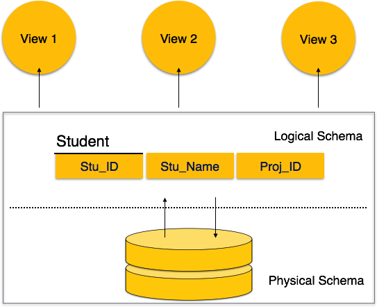
Fig 1 - Database schema

A database schema can be divided broadly into two categories −

●        Physical Database Schema−This schema pertains to the actual storage of data and its form of storage like files, indices, etc. It defines how the data will be stored in a secondary storage.

●        Logical Database Schema−This schema defines all the logical constraints that need to be applied on the data stored. It defines tables, views, and integrity constraints.

Database Instance

It is important that we distinguish these two terms individually. Database schema is the skeleton of database. It is designed when the database doesn't exist at all. Once the database is operational, it is very difficult to make any changes to it. A database schema does not contain any data or information.

A database instance is a state of operational database with data at any given time. It contains a snapshot of the database. Database instances tend to change with time. A DBMS ensures that its every instance (state) is in a valid state, by diligently following all the validations, constraints, and conditions that the database designers have imposed.

Q3) Explain in brief integrity constraints?

A3) Integrity Constraints

●        Integrity constraints are a set of rules. It is used to maintain the quality of information.

●        Integrity constraints ensure that the data insertion, updating, and other processes have to be performed in such a way that data integrity is not affected.

●        Thus, integrity constraint is used to guard against accidental damage to the database.

Types of Integrity Constraint

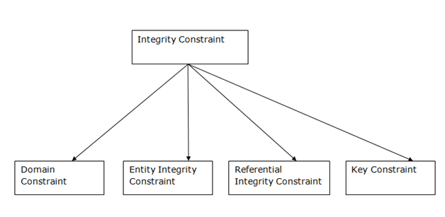
Fig 2 - Integrity Constraint

1. Domain constraints

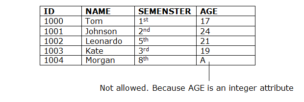
●        Domain constraints can be defined as the definition of a valid set of values for an attribute.

●        The data type of domain includes string, character, integer, time, date, currency, etc. The value of the attribute must be available in the corresponding domain.

Example:

2. Entity integrity constraints

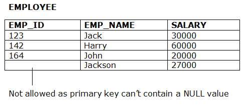
●        The entity integrity constraint states that primary key value can't be null.

●        This is because the primary key value is used to identify individual rows in relation and if the primary key has a null value, then we can't identify those rows.

●        A table can contain a null value other than the primary key field.

Example:

3. Referential Integrity Constraints

●        A referential integrity constraint is specified between two tables.

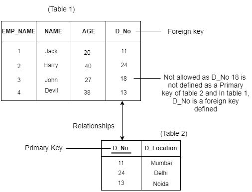
●        In the Referential integrity constraints, if a foreign key in Table 1 refers to the Primary Key of Table 2, then every value of the Foreign Key in Table 1 must be null or be available in Table 2.

Example:

4. Key constraints

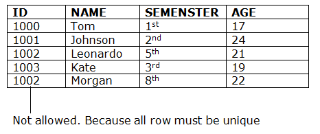
●        Keys are the entity set that is used to identify an entity within its entity set uniquely.

●        An entity set can have multiple keys, but out of which one key will be the primary key. A primary key can contain a unique and null value in the relational table.

Example:

Q4) What is Foreign Key in DBMS?

A4) Foreign key

A foreign key is different from a super key, candidate key or primary key because a foreign key is the one that is used to link two tables together or create connectivity between the two.

Here, in this section, we will discuss foreign key, its use and look at some examples that will help us to understand the working and use of the foreign key. We will also see its practical implementation on a database, i.e., creating and deleting a foreign key on a table.

What is a Foreign Key

A foreign key is the one that is used to link two tables together via the primary key. It means the columns of one table points to the primary key attribute of the other table. It further means that if any attribute is set as a primary key attribute will work in another table as a foreign key attribute. But one should know that a foreign key has nothing to do with the primary key.

Use of Foreign Key

The use of a foreign key is simply to link the attributes of two tables together with the help of a primary key attribute. Thus, it is used for creating and maintaining the relationship between the two relations.

Example of Foreign Key

Let's discuss an example to understand the working of a foreign key.

Consider two tables Student and Department having their respective attributes as shown in the below table structure:

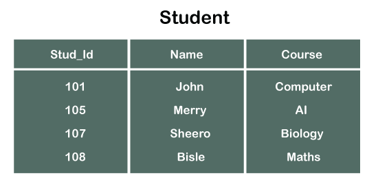
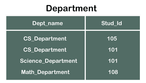
In the tables, one attribute, you can see, is common, that is Stud_Id, but it has different key constraints for both tables. In the Student table, the field Stud_Id is a primary key because it is uniquely identifying all other fields of the Student table. On the other hand, Stud_Id is a foreign key attribute for the Department table because it is acting as a primary key attribute for the Student table. It means that both the Student and Department table are linked with one another because of the Stud_Id attribute.

In the below-shown figure, you can view the following structure of the relationship between the two tables.

Note: Referential Integrity in DBMS is developed from the concept of the foreign key. It is clear that a primary key is an alone existing key and a foreign key always reference to a primary key in some other table, in which the table that contains the primary key is known as the referenced table or parent table for the other table that is having the foreign key.

Q5) Create Foreign Key constraint with an example?

A5)

On CREATE TABLE

Below is the syntax that will make us learn the creation of a foreign key in a table:

1. CREATE TABLE Department (  
2.    Dept_name varchar (120) NOT NULL,  
3.    Stud_Id int,  
4.      FOREIGN KEY (Stud_Id) REFERENCES Student (Stud_Id)  
5. );  

So, in this way, we can set a foreign key for a table in the MYSQL database.

In case of creating a foreign key for a table in SQL or Oracle server, the following syntax will work:

1. CREATE TABLE Department (  
2.    Dept_name varchar (120) NOT NULL,  
3.    Stud_Id int FOREIGN KEY REFERENCES Student (Stud_Id)  
4. );  

On ALTER TABLE

Following is the syntax for creating a foreign key constraint on ALTER TABLE:

1. ALTER TABLE Department  
2. ADD FOREIGN KEY (Stud_Id) REFERENCES Student (Stud_Id);  

Q6) What is relational algebra and what are its types give examples also?

A6) Relational algebra is a procedural query language. It gives a step by step process to obtain the result of the query. It uses operators to perform queries.

Types of Relational operation

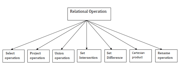
Fig 3 - Relational operation

1. Select Operation:

●        The select operation selects tuples that satisfy a given predicate.

●        It is denoted by sigma (σ).

Notation:  σ p(r)  

Where:

σ is used for selection prediction

r is used for relation

p is used as a propositional logic formula which may use connectors like: AND OR

And NOT. These relational can use as relational operators like =, ≠, ≥, <, >, ≤.

For example: LOAN Relation

Input:

1. σ BRANCH_NAME="perryride" (LOAN)  

Output:

2. Project Operation:

●        This operation shows the list of those attributes that we wish to appear in the result. Rest of the attributes are eliminated from the table.

●        It is denoted by ∏.

Notation: ∏ A1, A2, An (r)   

Where

A1, A2, A3 is used as an attribute name of relation r.

Example: CUSTOMER RELATION

Input:

1. ∏ NAME, CITY (CUSTOMER)  

Output:

3. Union Operation:

●        Suppose there are two tuples R and S. The union operation contains all the tuples that are either in R or S or both in R & S.

●        It eliminates the duplicate tuples. It is denoted by ∪.

Notation: R ∪ S   

A union operation must hold the following condition:

●        R and S must have the attribute of the same number.

●        Duplicate tuples are eliminated automatically.

Example:

DEPOSITOR RELATION

BORROW RELATION

Input:

1. ∏ CUSTOMER_NAME (BORROW) ∪ ∏ CUSTOMER_NAME (DEPOSITOR)  

Output:

4. Set Intersection:

●        Suppose there are two tuples R and S. The set intersection operation contains all tuples that are in both R & S.

●        It is denoted by intersection ∩.

Notation: R ∩ S   

Example: Using the above DEPOSITOR table and BORROW table

Input:

1. ∏ CUSTOMER_NAME (BORROW) ∩ ∏ CUSTOMER_NAME (DEPOSITOR)  

Output:

5. Set Difference:

●        Suppose there are two tuples R and S. The set intersection operation contains all tuples that are in R but not in S.

●        It is denoted by intersection minus (-).

Notation: R - S  

Example: Using the above DEPOSITOR table and BORROW table

Input:

1. ∏ CUSTOMER_NAME (BORROW) - ∏ CUSTOMER_NAME (DEPOSITOR)  

Output:

6. Cartesian product

●        The Cartesian product is used to combine each row in one table with each row in the other table. It is also known as a cross product.

●        It is denoted by X.

Notation: E X D  

Example:

EMPLOYEE

DEPARTMENT

Input:

1. EMPLOYEE X DEPARTMENT  

Output:

7. Rename Operation:

The rename operation is used to rename the output relation. It is denoted by rho (ρ).

Example: We can use the rename operator to rename STUDENT relation to STUDENT1.

ρ(STUDENT1, STUDENT)  

Q7) Explain join operation and its different types with examples?

A7) A Join operation combines related tuples from different relations, if and only if a given join condition is satisfied. It is denoted by ⋈.

Example:

EMPLOYEE

SALARY

1. Operation: (EMPLOYEE ⋈ SALARY)   

Result:

Types of Join operations:

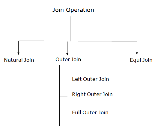
Fig 4 – Join Operation

1. Natural Join:

●        A natural join is the set of tuples of all combinations in R and S that are equal on their common attribute names.

●        It is denoted by ⋈.

Example: Let's use the above EMPLOYEE table and SALARY table:

Input:

1. ∏EMP_NAME, SALARY (EMPLOYEE ⋈ SALARY)  

Output:

2. Outer Join:

The outer join operation is an extension of the join operation. It is used to deal with missing information.

Example:

EMPLOYEE

FACT_WORKERS

Input:

1. (EMPLOYEE ⋈ FACT_WORKERS)  

Output:

An outer join is basically of three types:

1. Left outer join
2. Right outer join
3. Full outer join

a. Left outer join:

●        Left outer join contains the set of tuples of all combinations in R and S that are equal on their common attribute names.

●        In the left outer join, tuples in R have no matching tuples in S.

●        It is denoted by ⟕.

Example: Using the above EMPLOYEE table and FACT_WORKERS table

Input:

1. EMPLOYEE ⟕ FACT_WORKERS   

b. Right outer join:

●        Right outer join contains the set of tuples of all combinations in R and S that are equal on their common attribute names.

●        In right outer join, tuples in S have no matching tuples in R.

●        It is denoted by ⟖.

Example: Using the above EMPLOYEE table and FACT_WORKERS Relation

Input:

1. EMPLOYEE ⟖ FACT_WORKERS  

Output:

c. Full outer join:

●        Full outer join is like a left or right join except that it contains all rows from both tables.

●        In full outer join, tuples in R that have no matching tuples in S and tuples in S that have no matching tuples in R in their common attribute name.

●        It is denoted by ⟗.

Example: Using the above EMPLOYEE table and FACT_WORKERS table

Input:

1. EMPLOYEE ⟗ FACT_WORKERS  

Output:

3. Equijoin:

It is also known as an inner join. It is the most common join. It is based on matched data as per the equality condition. The equi join uses the comparison operator(=).

Example:

CUSTOMER RELATION

PRODUCT

Input:

1. CUSTOMER ⋈ PRODUCT    

Output:

Q8) What is relational calculus and what are its types explained with examples?

A8) Relational Calculus

●        Relational calculus is a non-procedural query language. In the non-procedural query language, the user is concerned with the details of how to obtain the end results.

●        The relational calculus tells what to do but never explains how to do.

Types of Relational calculus:

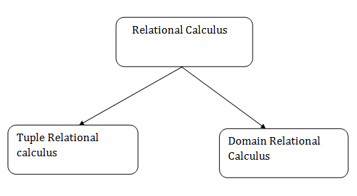
Fig 5 - Relational calculus

1. Tuple Relational Calculus (TRC)

●        The tuple relational calculus is specified to select the tuples in a relation. In TRC, filtering variable uses the tuples of a relation.

●        The result of the relation can have one or more tuples.

Notation:

1. {T | P (T)}   or {T | Condition (T)}   

Where

T is the resulting tuples

P(T) is the condition used to fetch T.

For example:

1. { T.name | Author(T) AND T.article = 'database' }  

OUTPUT: This query selects the tuples from the AUTHOR relation. It returns a tuple with 'name' from Author who has written an article on 'database'.

TRC (tuple relation calculus) can be quantified. In TRC, we can use Existential (∃) and Universal Quantifiers (∀).

For example:

1. { R| ∃T ∈ Authors(T.article='database' AND R.name=T.name)}  

Output: This query will yield the same result as the previous one.

2. Domain Relational Calculus (DRC)

●        The second form of relation is known as Domain relational calculus. In domain relational calculus, filtering variable uses the domain of attributes.

●        Domain relational calculus uses the same operators as tuple calculus. It uses logical connectives ∧ (and), ∨ (or) and ┓ (not).

●        It uses Existential (∃) and Universal Quantifiers (∀) to bind the variable.

Notation:

1. { a1, a2, a3, ..., an | P (a1, a2, a3, ... ,an)}  

Where

a1, a2 are attributes

P stands for formula built by inner attributes

For example:

1. {< article, page, subject > |  ∈ javatpoint ∧ subject = 'database'}  

Output: This query will yield the article, page, and subject from the relational javatpoint, where the subject is a database.

Q9) Explain Indexing in DBMS with examples

A9) Indexing in DBMS

●        Indexing is used to optimize the performance of a database by minimizing the number of disk accesses required when a query is processed.

●        The index is a type of data structure. It is used to locate and access the data in a database table quickly.

Index structure:

Indexes can be created using some database columns.

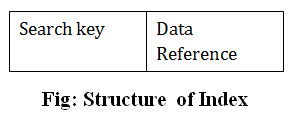
Fig 6 – Structure of Index

●        The first column of the database is the search key that contains a copy of the primary key or candidate key of the table. The values of the primary key are stored in sorted order so that the corresponding data can be accessed easily.

●        The second column of the database is the data reference. It contains a set of pointers holding the address of the disk block where the value of the particular key can be found.

Indexing Methods

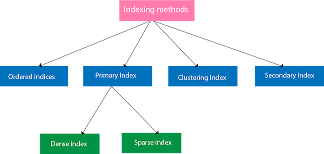
Fig 7 – Indexing Methods

Ordered indices

The indices are usually sorted to make searching faster. The indices which are sorted are known as ordered indices.

Example: Suppose we have an employee table with thousands of record and each of which is 10 bytes long. If their IDs start with 1, 2, 3....and so on and we have to search student with ID-543.

●        In the case of a database with no index, we have to search the disk block from starting till it reaches 543. The DBMS will read the record after reading 543*10=5430 bytes.

●        In the case of an index, we will search using indexes and the DBMS will read the record after reading 542*2= 1084 bytes which are very less compared to the previous case.

Primary Index

●        If the index is created on the basis of the primary key of the table, then it is known as primary indexing. These primary keys are unique to each record and contain 1:1 relation between the records.

●        As primary keys are stored in sorted order, the performance of the searching operation is quite efficient.

●        The primary index can be classified into two types: Dense index and Sparse index.

Dense index

●        The dense index contains an index record for every search key value in the data file. It makes searching faster.

●        In this, the number of records in the index table is same as the number of records in the main table.

●        It needs more space to store index record itself. The index records have the search key and a pointer to the actual record on the disk.

Fig 8 – Dense Index

Sparse index

●        In the data file, index record appears only for a few items. Each item points to a block.

●        In this, instead of pointing to each record in the main table, the index points to the records in the main table in a gap.

Fig 9 – Sparse Index

Clustering Index

●        A clustered index can be defined as an ordered data file. Sometimes the index is created on non-primary key columns which may not be unique for each record.

●        In this case, to identify the record faster, we will group two or more columns to get the unique value and create index out of them. This method is called a clustering index.

●        The records which have similar characteristics are grouped, and indexes are created for these group.

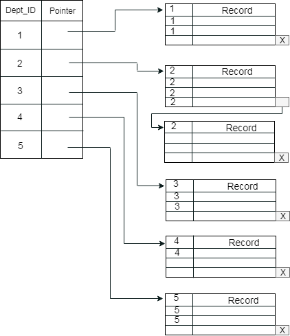
Example: suppose a company contains several employees in each department. Suppose we use a clustering index, where all employees which belong to the same Dept_ID are considered within a single cluster, and index pointers point to the cluster as a whole. Here Dept Id is a non-unique key.

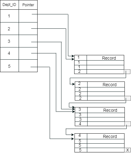
The previous schema is little confusing because one disk block is shared by records which belong to the different cluster. If we use separate disk block for separate clusters, then it is called better technique.

Secondary Index

In the sparse indexing, as the size of the table grows, the size of mapping also grows. These mappings are usually kept in the primary memory so that address fetch should be faster. Then the secondary memory searches the actual data based on the address got from mapping. If the mapping size grows then fetching the address itself becomes slower. In this case, the sparse index will not be efficient. To overcome this problem, secondary indexing is introduced.

In secondary indexing, to reduce the size of mapping, another level of indexing is introduced. In this method, the huge range for the columns is selected initially so that the mapping size of the first level becomes small. Then each range is further divided into smaller ranges. The mapping of the first level is stored in the primary memory, so that address fetch is faster. The mapping of the second level and actual data are stored in the secondary memory (hard disk).

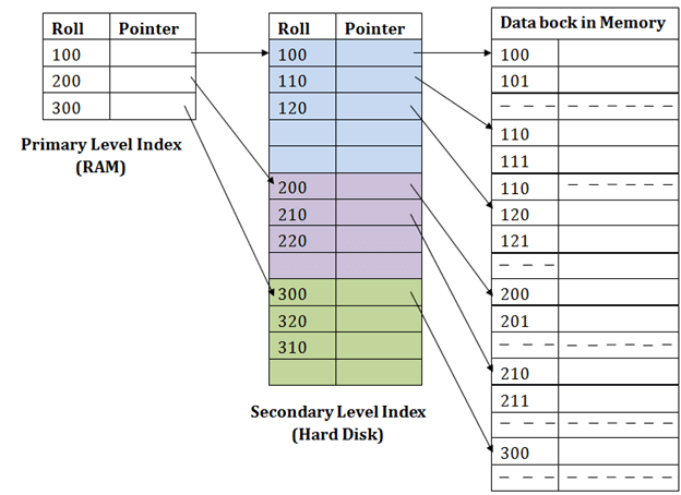
Fig 10 – Secondary Index

For example:

●        If you want to find the record of roll 111 in the diagram, then it will search the highest entry which is smaller than or equal to 111 in the first level index. It will get 100 at this level.

●        Then in the second index level, again it does max (111) <= 111 and gets 110. Now using the address 110, it goes to the data block and starts searching each record till it gets 111.

●        This is how a search is performed in this method. Inserting, updating or deleting is also done in the same manner.

Q10) What is functional dependency?

A10) Functional Dependency

Functional dependency (FD) is a set of constraints between two attributes in a relation. Functional dependency says that if two tuples have same values for attributes A1, A2,..., An, then those two tuples must have to have same values for attributes B1, B2, ..., Bn.

Functional dependency is represented by an arrow sign (→) that is, X→Y, where X functionally determines Y. The left-hand side attributes determine the values of attributes on the right-hand side.

Armstrong's Axioms

If F is a set of functional dependencies then the closure of F, denoted as F+, is the set of all functional dependencies logically implied by F. Armstrong's Axioms are a set of rules, that when applied repeatedly, generates a closure of functional dependencies.

●        Reflexive rule− If alpha is a set of attributes and beta is_subset_of alpha, then alpha holds beta.

●        Augmentation rule− If a → b holds and y is attribute set, then ay → by also holds. That is adding attributes in dependencies, does not change the basic dependencies.

●        Transitivity rule−Same as transitive rule in algebra, if a → b holds and b → c holds, then a → c also holds. a→ b is called as a functionally that determines b.

Trivial Functional Dependency

●        Trivial− If a functional dependency (FD) X → Y holds, where Y is a subset of X, then it is called a trivial FD. Trivial FDs always hold.

●        Non-trivial− If an FD X → Y holds, where Y is not a subset of X, then it is called a non-trivial FD.

●        Completely non-trivial− If an FD X → Y holds, where x intersect Y = Φ, it is said to be a completely non-trivial FD.

Q11) Explain normalization in database and what are the different types of normalization

A11) Normalization

If a database design is not perfect, it may contain anomalies, which are like a bad dream for any database administrator. Managing a database with anomalies is next to impossible.

●        Update anomalies− If data items are scattered and are not linked to each other properly, then it could lead to strange situations. For example, when we try to update one data item having its copies scattered over several places, a few instances get updated properly while a few others are left with old values. Such instances leave the database in an inconsistent state.

●        Deletion anomalies−We tried to delete a record, but parts of it was left undeleted because of unawareness, the data is also saved somewhere else.

●        Insert anomalies−We tried to insert data in a record that does not exist at all.

Normalization is a method to remove all these anomalies and bring the database to a consistent state.

First Normal Form

First Normal Form is defined in the definition of relations (tables) itself. This rule defines that all the attributes in a relation must have atomic domains. The values in an atomic domain are indivisible units.

Fig 11 – 1NF

We rearrange the relation (table) as below, to convert it to First Normal Form.

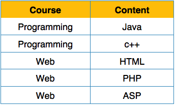
Fig 12 - Rearrange the relation 1NF

Each attribute must contain only a single value from its pre-defined domain.

Second Normal Form

Before we learn about the second normal form, we need to understand the following −

●        Prime attribute−An attribute, which is a part of the candidate-key, is known as a prime attribute.

●        Non-prime attribute−An attribute, which is not a part of the prime-key, is said to be a non-prime attribute.

If we follow second normal form, then every non-prime attribute should be fully functionally dependent on prime key attribute. That is, if X →A holds, then there should not be any proper subset Y of X, for which Y → A also holds true.

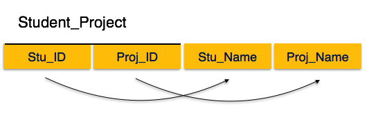
Fig 13 – 2 NF

We see here in Student_Project relation that the prime key attributes are Stu_ID and Proj_ID. According to the rule, non-key attributes, i.e. Stu_Name and Proj_Name must be dependent upon both and not on any of the prime key attribute individually. But we find that Stu_Name can be identified by Stu_ID and Proj_Name can be identified by Proj_ID independently. This is called partial dependency, which is not allowed in Second Normal Form.

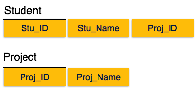
Fig 14 - Partial dependency

We broke the relation in two as depicted in the above picture. So there exists no partial dependency.

Third Normal Form

For a relation to be in Third Normal Form, it must be in Second Normal form and the following must satisfy −

●        No non-prime attribute is transitively dependent on prime key attribute.

●        For any non-trivial functional dependency, X → A, then either −

• X is a superkey or,
• A is prime attribute.

Fig 15 – 3 NF

We find that in the above Student_detail relation, Stu_ID is the key and only prime key attribute. We find that City can be identified by Stu_ID as well as Zip itself. Neither Zip is a superkey nor is City a prime attribute. Additionally, Stu_ID→ Zip → City, so there exists transitive dependency.

To bring this relation into third normal form, we break the relation into two relations as follows −

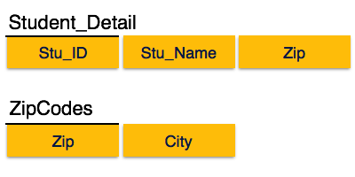
Boyce-Codd Normal Form

Boyce-Codd Normal Form (BCNF) is an extension of Third Normal Form on strict terms. BCNF states that −

●        For any non-trivial functional dependency, X → A, X must be a super-key.

In the above image, Stu_ID is the super-key in the relation Student_Detail and Zip is the super-key in the relation ZipCodes. So,

Stu_ID→Stu_Name, Zip

And

Zip → City

Which confirms that both the relations are in BCNF.

Q12) Define hash index?

A12) A hash index is created by taking the prefix of a complete hash value. A depth number is assigned to each hash index to indicate how many bits are used to compute a hash function. These bits can be used to address up to 2n buckets. When all of these bits have been spent, the depth value is increased linearly, and the buckets are divided in half.

A hash index is a technique for expediting the search process. Traditional indexes require you to scan each row to ensure that your query is successful. This isn't the case with hash indexes, though!

Each index key comprises only one row of table data and uses the hashing indexing process to assign them a unique memory address, removing all other keys with duplicate values before locating what they're seeking for.

One of the various methods to organise data in a database is to use hash indexes. They work by collecting user input and using it as a key for disc storage. These keys, also known as hash values, might be anything from string lengths to input characters.

When querying specific inputs with specified features, hash indexes are most typically employed. It may be, for example, locating all A-letters that are higher than 10 cm. By constructing a hash index function, you can do it rapidly.

The PostgreSQL database system includes hash indexes. This technology was created to boost speed and efficiency. Hash indexes can be combined with other index types such as B-tree and GiST.

A hash index divides keys into smaller portions called buckets, each of which is given an integer ID number so that it may be conveniently retrieved when looking for a key's placement in the hash table. The buckets are stored sequentially on a disk so that the data they contain can be quickly accessed.

Q13) Write the advantages and disadvantages of hash index?

A13) Advantages

The fundamental benefit of employing hash indexes is that they provide for quick access to records when searching by key value. It is frequently used in queries that have an equality condition. Hash benchmarks also don't take up a lot of storage space. As a result, it is a useful tool, although it is not without flaws.

Disadvantages

Hash indexes are a relatively new indexing mechanism that has the potential to improve performance significantly. You can think of them as a binary search tree with a twist (BSTs).

Hash indexes work by grouping data into buckets depending on their hash values, allowing for quick and efficient data retrieval. They will always be in good working order.

Duplicate keys, on the other hand, cannot be stored in a bucket. As a result, some overhead will always exist. However, thus far, the benefits of employing hash indexes exceed the disadvantages.

Q14) What do you mean by bitmap index?

A14) Bitmap indexing is a sort of database indexing in which bitmaps are used. This strategy is employed in large databases where columns have a low cardinality and are regularly used in queries.

It's a sort of indexing that's based on a single key. It is, however, designed to swiftly execute searches on numerous keys. Before we can use bitmap indexing, we need to arrange the records in a sequential order. It simplifies the process of retrieving a specific record from the block. It is also simple to allocate them in a file's block.

The bit is the lowest unit for representing data with values of 0 or 1. It's the bit arrays that perform bitwise logical operations on bitmaps to answer queries. Indexing is a data structure that arranges data according to a set of rules. When a column has a low cardinality and is frequently used in a query, this bitmap indexing approach is used in large databases. Low cardinality columns are those that have a small number of unique values. We will explore why it is necessary, as well as its applications, benefits, and drawbacks in today's IT world.

It is used in data warehousing applications with a large amount of data and complex queries but low-level transactions. It aids in reducing response time for complex queries, space reduction compared to other indexing techniques, increased hardware performance with fewer CPUs and memory, and effective maintenance for such applications. Low cardinality columns have multiple distinct values, either absolute or proportional to the amount of data entries. Low cardinality can also take on Boolean values, such as true or false.

The index gives you a list of all the rows in a table that have a specific key value. A conventional index keeps a list of row ids for each key in the same row as the key-value row, but a key-value index saves each key-value instead of its list of row ids.

Structure of Bitmap

The words 'bitmap' are made up of the words 'bit' and'map.' In a computer system, a bit is the smallest unit of data. A map is a visual representation of how things are organised. As a result, a bitmap is essentially an array of bits that have been mapped. Each attribute in a relation has its own bitmap for its value. A bitmap has enough bits to number each record in a block.

Consider the Student record relation, where we want to find out which female and male students have an English score of greater than 40. The gender bitmaps are shown in the figure below.

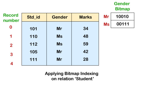
When the value of a record is set to Mr, the bitmap's ithbit will be set to 1. All remaining bits in the bitmap for Mr will be set to 0. In the case of female students, the identical procedure is followed. If the value is set to Ms for a particular j record, the jth bit in the bitmap will be set to 1. For Ms, all other bits will be set to 0. Now, a user just needs to read all the records in the relation to retrieve either a single or all records for female students or male students, i.e., value as Mr or Ms. Select the required records for Mr. Or Ms. After reading.

The bitmap indexing, on the other hand, makes it difficult to swiftly choose entries. However, it allows users to read and select only the records they need. As can be seen in the sample above, the user only picked the required records for female or male students.

Q15) Write the advantages and disadvantages of bitmap index?

A15) Advantages

●      When fewer cardinality columns are utilised in querying often, it aids in speedier data retrieval.

●      Even if the table has a large number of records, it is efficient.

●      Incorporating table columns into insertion, updating, and deletion actions would be far more efficient.

●      When running a query, multiple indices can be combined.

●      On a temporary table, a Bitmap join index can be built.

Disadvantages

●      For databases with fewer records, bitmap indexing is ineffective because DBMSs demand a full scan of the table instead of using bitmap indexing.

●      Multiple insertions, updates, and deletions from various users can result in a stalemate.

●      Bitmap indexing costs time to perform DML operations because it takes time to complete the transaction and update the bitmap index.

●      Maintaining a large number of records can be time consuming.

●      If the user inputs a new record, it must be changed throughout, which is time-consuming and complicated.

●      When utilising the bitmap join index, only one table can be modified by many transactions.

●      The table's UNIQUE property prevents it from being created.