Unit - 1

Digital Communication Concept

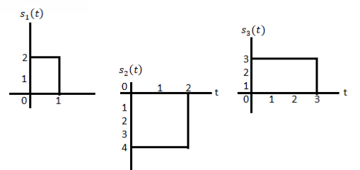
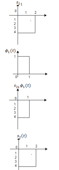
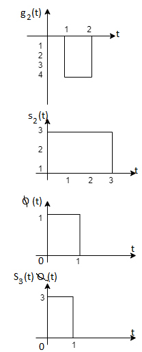
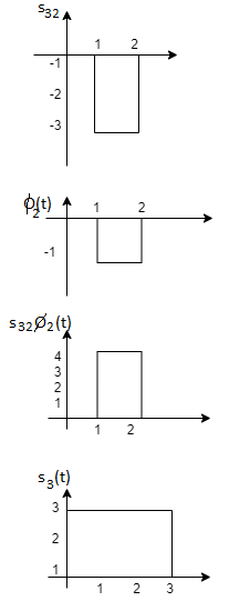
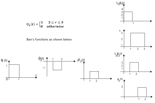
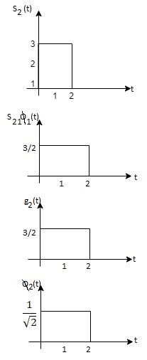
Q1) Using the Gram Schmitt orthogonalization procedure, find a set of orthonormal ban’s functions represent the tree signals as shown in figure.

A1)

All the three signals are not linear combination of each other hence they are linearly independent. Hence, we require three ban’s function.

To obtain

Energy of

To obtain

To obtain

Q2) Consider the signals andas given below. Find an orthonormal basis for phase set of signals using Grammar schimdt orthogonalisation procedure.

Fig 1. Sketch of and

A2)

From the above figures . This means all four signals are not linearly independent. Gram-schmidt orthogonalisation procedure is carried out for a subset which is linearly independent. Here are linearly independent. Hence, we will determine orthonormal.

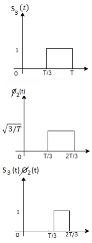
To obtain

Energy of is

We know that

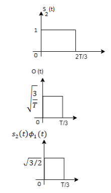
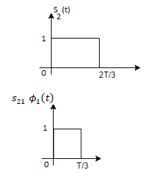
To obtain

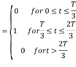
From the above figure the intermediate function can be defined as

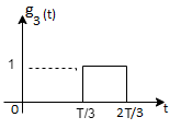
Energy of will be

Now

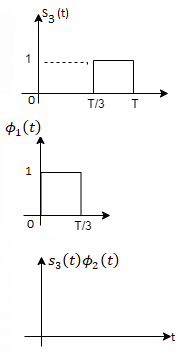
To obtain

We know that the generalized equation for Gram Schmitt procedure

With N=3

We know that

Since, there is no overlap between and

Here

We know that

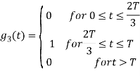
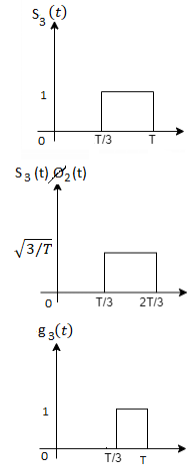
Figure below shows orthonormal basis function

Q3) Three signals are shown in fig. Apply Gram-schmidt procedure to obtain an orthonormal basis for the signals. Express signals in terms of orthonormal basis function.

A3)

i) To obtain orthonormal basis function

Here

Hence, we will obtain basis solution for and only.

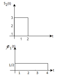
To obtain

Energy of is

We know that

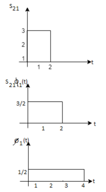
To obtain

Q4) What are random signals?

A4) Random signals and noise are present in several engineering systems. Practical signals seldom lend themselves to a nice mathematical deterministic description. It is partly a consequence of the chaos that is produced by nature. However, chaos can also be man-made, and one can even state that chaos is a condition sine qua non to be able to transfer information. Signals that are not random in time but predictable contain no information, as was concluded by Shannon in his famous communication theory.

A (one-dimensional) random process is a (scalar) function y(t), where t is usually time, for which the future evolution is not determined uniquely by any set of initial data or at least by any set that is knowable to you and me. In other words, random process" is just a fancy phrase that means unpredictable function". Random processes y takes on a continuum of values ranging over some interval, often but not always - to +. The generalization to y's with discrete (e.g., integral) values is straightforward

Examples of random processes are:

(i) The total energy E(t) in a cell of gas that is in contact with a heat bath;

(ii) The temperature T(t) at the corner of Main Street and Center Street in Logan, Utah;

(iii) The earth-longitude (t) of a specific oxygen molecule in the earth's atmosphere.

One can also deal with random processes that are vector or tensor functions of time. Ensembles of random processes. Since the precise time evolution of a random process is not predictable, if one wishes to make predictions one can do so only probabilistically. The foundation for probabilistic predictions is an ensemble of random processes |i.e., a collection of a huge number of random processes each of which behaves in its own, unpredictable way. The probability density function describes the general distribution of the magnitude of the random process, but it gives no information on the time or frequency content of the process. Ensemble averaging and Time averaging can be used to obtain the process properties.

Q5) Explain correlation and covariance function?

A5) Correlation

The covariance has units (units of X times units of Y), and thus it can be difficult to assess how strongly related two quantities are.  The correlation coefficient is a dimensionless quantity that helps to assess this.

The correlation coefficient between X and Y normalizes the covariance such that the resulting statistic lies between -1 and 1.  The Pearson correlation coefficient is

The correlation matrix for X and Y is

Covariance

If we have two samples of the same size, X_i, and Y_i, where i=1,…,n, then the covariance is an estimate of how variation in X is related to variation in Y.  The covariance is defined as

Where mu_X is the mean of the X sample, and mu_Y is the mean of the Y sample.  Negative covariance means that smaller X tend to be associated with larger Y (and vice versa).  Positive covariance means that larger/smaller X are associated with larger/smaller Y.  Note that the covariance of X and Y is exactly the same as the covariance of Y and X.  Also note that the covariance of X with itself is the variance of X.  The covariance matrix for X and Y is thus

Q6) What is meant by ergodic process?

A6)

•         In econometrics and signal processing, a stochastic process is said to be ergodic if its statistical properties can be deduced from a single, sufficiently long, random sample of the process.

•         The reasoning is that any collection of random samples from a process must represent the average statistical properties of the entire process.

•         In other words, regardless of what the individual samples are, a birds-eye view of the collection of samples must represent the whole process.

•         Conversely, a process that is not ergodic is a process that changes erratically at an inconsistent rate.

Q7) Let X(t)be a zero-mean WSS process with RX(τ)=e−|τ|. X(t)is input to an LTI system with

|H(f)|=√ (1+4π2f2)   |f|<2

= 0            otherwise,

Let Y(t) be the output.

1. Find μY(t)=E[Y(t)]
2. Find RY(τ)
3. Find E[Y(t)2]

A7) Note that since X(t)is WSS, X(t)and Y(t)are jointly WSS, and therefore Y(t)is WSS.

1. To find μY(t), we can write

μY=μXH(0) =0*1= 0

b.     To find RY(τ), we first find SY(f)

SY(f)=SX(f)|H(f)|2

From Fourier transform tables, we can see that

SX(f)=F{e−|τ|} =2/(1+(2πf)2)

Then, we can find SY(f)as

SY(f)=SX(f)|H(f)|2

=2|f|<2

= 0 otherwise

We can now find RY(τ)by taking the inverse Fourier transform of SY(f)

RY(τ)=8sinc(4τ),

Where

Sinc(f)=sin(πf)/πf

c.      We have

E[Y(t)2] = RY (0) =8.

Q8) A factory has two machines A and B making 60% and 40% respectively of the total production. Machine A produces 3% defective items, and B produces 5% defective items. Find the probability that a given defective part came from A.

A8)

We consider the following events:

A: Selected item comes from A.

B: Selected item comes from B.

D: Selected item is defective.

We are looking for . We know:

Now,

So we need

Since, D is the union of the mutually exclusive events and (the entire sample space is the union of the mutually exclusive events A and B)

Q9) Explain LTI system with random inputs?

A9) LTI Systems with Random Inputs:

Consider an LTI system with impulse response h(t). Let X(t) be a WSS random process. If X(t) is the input of the system, then the output, Y(t), is also a random process. More specifically, we can write

Y(t)=h(t)∗X(t)=

Here, our goal is to show that X(t) and Y(t) are jointly WSS processes. Let's first start by calculating the mean function of Y(t), μY(t). We have

μY(t)=E[Y(t)]

=E []

=

=

=μX

We note that μY(t)is not a function of t, so we can write

μY(t)=μY=μX.

Let's next find the cross-correlation function, RXY(t1, t2).

We have

RXY(t1, t2) =E[X(t1)Y(t2)]=E[X(t1)]

=E[

=

=

=(since X(t) is WSS).

We note that RXY(t1,t2)is only a function of τ=t1−t2, so we may write

RXY(τ)=

=h(τ)∗RX(−τ)

=h(−τ)∗RX(τ).

Similarly, you can show that

RY(τ)=h(τ)∗h(−τ)∗RX(τ).

From the above results we conclude that X(t)and Y(t)are jointly WSS.

Q10) Explain central limit theorem?

A10)

The central limit theorem (CLT) is one of the most important results in probability theory.

It states that, under certain conditions, the sum of a large number of random variables is approximately normal.

Here, we state a version of the CLT that applies to i.i.d. Random variables. Suppose that X1, X2 , ... , Xn are i.i.d. Random variables with expected values EXi=μ<∞ and variance Var(Xi)=σ2<∞. Then the sample mean X¯¯=X1+X2+...+Xnn has mean EX¯=μ and variance Var(X¯)=σ2n.

= μ

=

Where,
μ = Population mean

σ = Population standard deviation

μx¯= Sample mean

σx¯ = Sample standard deviation

n = Sample size

How to Apply The Central Limit Theorem (CLT)

Here are the steps that we need in order to apply the CLT:

1.Write the random variable of interest, Y, as the sum of n i.i.d. Random variable Xi's:

Y=X1+X2+...+Xn.

2.Find EY and Var(Y) by noting that

EY=nμ,Var(Y)=nσ2,

Where μ=EXi and σ2=Var(Xi).

3.According to the CLT, conclude that

Y−EY/ √Var(Y)=Y−nμ/ √nσ is approximately standard normal; thus, to find P(y1≤Y≤y2), we can write

P(y1≤Y≤y2)=P(y1−nμ/√nσ≤Y−nμ/√nσ≤y2−nμ/√nσ)

≈Φ(y2−nμ/ √nσ)−Φ(y1−nμ/√nσ).

Q11) In a communication system each data packet consists of 1000 bits. Due to the noise, each bit may be received in error with probability 0.1. It is assumed bit errors occur independently. Find the probability that there are more than 120 errors in a certain data packet.

A11)

Let us define Xi as the indicator random variable for the ith bit in the packet. That is, Xi=1 if the ith bit is received in error, and Xi=0 otherwise. Then the Xi's are i.i.d. And Xi∼Bernoulli(p=0.1).

If Y is the total number of bit errors in the packet, we have

Y=X1+X2+...+Xn.

Since Xi∼Bernoulli(p=0.1), we have

EXi=μ=p=0.1,Var(Xi)=σ2=p(1−p)=0.09

Using the CLT, we have

P(Y>120)=P(Y−nμ/ √nσ>120−nμ/√nσ)

=P(Y−nμ/√nσ>120−100/ √90)

≈1−Φ(20/√90)=0.0175

Q12) Explain the block diagram of digital communication system?

A12)

The elements which form a digital communication system is represented by the following block diagram for the ease of understanding.

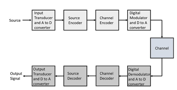
Fig 2. Elements of Digital Communication System

Following are the sections of the digital communication system.

Source

The source can be an analog signal. 

Example: A Sound signal

Input Transducer

This is a transducer which takes a physical input and converts it to an electrical signal. This block also consists of an analog to digital converter where a digital signal is needed for further processes.

A digital signal is generally represented by a binary sequence.

Source Encoder

The source encoder compresses the data into minimum number of bits. This process helps in effective utilization of the bandwidth. It removes the redundant bits unnecessary excess bits, i.e., zeroes.

Channel Encoder

The channel encoder, does the coding for error correction. During the transmission of the signal, due to the noise in the channel, the signal may get altered and hence to avoid this, the channel encoder adds some redundant bits to the transmitted data. These are the error correcting bits.

Digital Modulator

The signal to be transmitted is modulated here by a carrier. The signal is also converted to analog from the digital sequence, in order to make it travel through the channel or medium.

Channel

The channel or a medium, allows the analog signal to transmit from the transmitter end to the receiver end.

Digital Demodulator

This is the first step at the receiver end. The received signal is demodulated as well as converted again from analog to digital. The signal gets reconstructed here.

Channel Decoder

The channel decoder, after detecting the sequence, does some error corrections. The distortions which might occur during the transmission, are corrected by adding some redundant bits. This addition of bits helps in the complete recovery of the original signal.

Source Decoder

The resultant signal is once again digitized by sampling and quantizing so that the pure digital output is obtained without the loss of information. The source decoder recreates the source output.

Output Transducer

This is the last block which converts the signal into the original physical form, which was at the input of the transmitter. It converts the electrical signal into physical output.

Output Signal

This is the output which is produced after the whole process.

Q13) Explain in detail about the signal space concept?

A13)

As in the case of vectors, we may develop a parallel treatment for a set of signals.

The inner product of two generally complex-valued signals x1(t) and x2(t) is denoted by <x1(t), x2(t)> and defined by

The signals are orthogonal if their inner product is zero. The norm of a signal is defined as

Where x is the energy in x(t). A set of m signal is orthonormal if they are orthogonal and their norms are all unity.

The Gram-Schmidt orthogonalization procedure can be used to construct a set of orthonormal waveforms from a set of finite energy signal waveforms: xi(t), 1 ≤ i ≤ m.

Once we have constructed the set of, say k, orthonormal waveforms {φk(t)}, we can express the signals {xi(t)} as linear combinations of the φk(t). Thus, we may write

Based on the above expression, each signal may be represented by the vector

x (i) = (xi,1, xi,2, . . . , xi,K ) T

Or, equivalently, as a point in the N-dimensional (in general, complex) signal space.

A set of M signals {xi(t)} can be represented by a set of M vectors {x (i)} in the N-dimensional space. The corresponding set of vectors is called the signal space representation, or constellation, of {xi(t)}.

• If the original signals are real, then the corresponding vector representations are in RK; and if the signals are complex, then the vector representations are in CK.

• Figure demonstrates the process of obtaining the vector equivalent from a signal (signal-to-vector mapping) and vice versa (vector-to signal mapping).

Fig 3. Vector to signal (a), and signal to vector (b) mappings

Q14) Explain geometric representation of signals?

A14)

Geometric representation of signals can provide a compact characterization of signals and can simplify analysis of their performance as modulation signals. Orthonormal bases are essential in geometry. Let {s1 (t), s2 (t), . . . , sM (t)} be a set of signals.

ψ1(t) = s1(t)/E1 where E1 =

s21 = < s2, ψ1 >=    and ψ2(t) = 1/2(s2(t) – s21(t) – s21ψ1)

2 =

ψk(t) = 1/2 ( sk(t) – )

k =

sm(t) =

The process continues until all of the M signals are exhausted. The results are N orthogonal signals with unit energy, {ψ1 (t), ψ2 (t), . . . , ψN (t)}. If the signals {s1 (t), . . . , sM (t)} are linearly independent, then N = M.

m ∈ {1, 2, . . . , M}

The M signals can be represented as

smn =< sm, ψn > and Em =

Q15) What are correlation receiver?

A15)

In other terms, the inner product is a correlation

But we want to build a receiver that does the minimum amount of calculation. If si(t) are non-orthogonal, then we can reduce the amount of correlation (and thus multiplication and addition) done in the receiver by instead, correlating with the basis functions, {φk(t)} N k=1. Correlation with the basis functions gives

x = [x1, x2, . . . , xN]T

Now that we’ve done these N correlations (inner products), we can compute the estimate of the received signal as

                                                       r(t) = bsi(t) + n(t)

                                                      n(t) = 0 and b = 1

                                                               x = ai

Where ai is the signal space vector for si(t).

Our signal set can be represented by the orthonormal basis functions, . Correlation with the basis functions gives

For k = 0 . . . K − 1. We denote vectors:

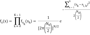
Hopefully, x and ai should be close since i was actually sent. In general, the pdf of x is multivariate Gaussian with each component xk independent, because

• xk = ai,k + nk
• ai,k is a deterministic constant
• The {nk} are i.i.d. Gaussian.

The joint pdf of x is

Q16) Explain in detail about matched filter receiver?

A16)

If a filter produces an output in such a way that it maximizes the ratio of output peak power to mean noise power in its frequency response, then that filter is called Matched filter.

Fig 4: Matched filter

Frequency Response Function of Matched Filter

The frequency response of the Matched filter will be proportional to the complex conjugate of the input signal’s spectrum. Mathematically, we can write the expression for frequency response function, H(f) of the Matched filter as −

H(f)=GaS∗(f)e−j2πft1    ………..1

Where,

Ga is the maximum gain of the Matched filter

S(f) is the Fourier transform of the input signal, s(t)

S∗(f) is the complex conjugate of S(f)

t1 is the time instant at which the signal observed to be maximum

In general, the value of Ga is considered as one. We will get the following equation by substituting Ga=1in Equation 1.

H(f)=S∗(f)e−j2πft1  ……..2

The frequency response function, H(f) of the Matched filter is having the magnitude of S∗(f)and phase angle of e−j2πft1, which varies uniformly with frequency.

Impulse Response of Matched Filter

In time domain, we will get the output, h(t) of Matched filter receiver by applying the inverse Fourier transform of the frequency response function, H(f).

h(t) =   .….3

Substitute, Equation 1 in Equation 3.

h(t) =

⇒ h(t) = ………4

We know the following relation.

S∗(f)=S(−f)                                   ……..5

Substitute, Equation 5 in Equation 4.

h(t) =

h(t) =

 h(t) = Gas(t1 – t)

In general, the value of Ga is considered as one. We will get the following equation by substituting Ga=1.

h(t)=s(t1−t)

The above equation proves that the impulse response of Matched filter is the mirror image of the received signal about a time instant t1. The following figures illustrate this concept.

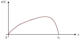
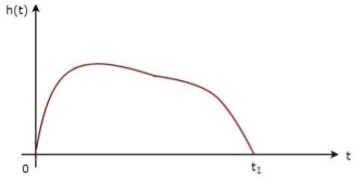
Fig 5: Impulse response of Matched filter 

The received signal, s(t) and the impulse response, h(t) of the matched filter corresponding to the signal, s(t) are shown in the above figures.

Unit - 1

Unit - 1

Unit - 1

Digital Communication Concept

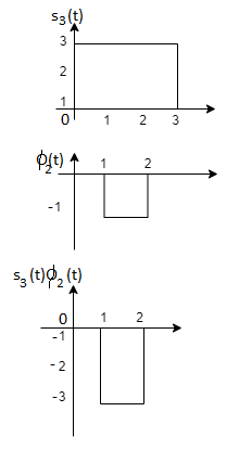
Q1) Using the Gram Schmitt orthogonalization procedure, find a set of orthonormal ban’s functions represent the tree signals as shown in figure.

A1)

All the three signals are not linear combination of each other hence they are linearly independent. Hence, we require three ban’s function.

To obtain

Energy of

To obtain

To obtain

Q2) Consider the signals andas given below. Find an orthonormal basis for phase set of signals using Grammar schimdt orthogonalisation procedure.

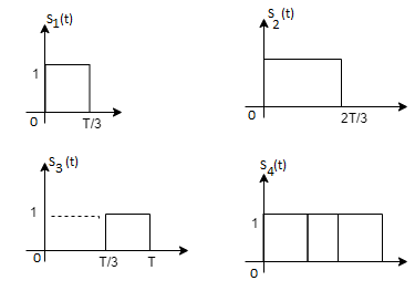
Fig 1. Sketch of and

A2)

From the above figures . This means all four signals are not linearly independent. Gram-schmidt orthogonalisation procedure is carried out for a subset which is linearly independent. Here are linearly independent. Hence, we will determine orthonormal.

To obtain

Energy of is

We know that

To obtain

From the above figure the intermediate function can be defined as

Energy of will be

Now

To obtain

We know that the generalized equation for Gram Schmitt procedure

With N=3

We know that

Since, there is no overlap between and

Here

We know that

Figure below shows orthonormal basis function

Q3) Three signals are shown in fig. Apply Gram-schmidt procedure to obtain an orthonormal basis for the signals. Express signals in terms of orthonormal basis function.

A3)

i) To obtain orthonormal basis function

Here

Hence, we will obtain basis solution for and only.

To obtain

Energy of is

We know that

To obtain

Q4) What are random signals?

A4) Random signals and noise are present in several engineering systems. Practical signals seldom lend themselves to a nice mathematical deterministic description. It is partly a consequence of the chaos that is produced by nature. However, chaos can also be man-made, and one can even state that chaos is a condition sine qua non to be able to transfer information. Signals that are not random in time but predictable contain no information, as was concluded by Shannon in his famous communication theory.

A (one-dimensional) random process is a (scalar) function y(t), where t is usually time, for which the future evolution is not determined uniquely by any set of initial data or at least by any set that is knowable to you and me. In other words, random process" is just a fancy phrase that means unpredictable function". Random processes y takes on a continuum of values ranging over some interval, often but not always - to +. The generalization to y's with discrete (e.g., integral) values is straightforward

Examples of random processes are:

(i) The total energy E(t) in a cell of gas that is in contact with a heat bath;

(ii) The temperature T(t) at the corner of Main Street and Center Street in Logan, Utah;

(iii) The earth-longitude (t) of a specific oxygen molecule in the earth's atmosphere.

One can also deal with random processes that are vector or tensor functions of time. Ensembles of random processes. Since the precise time evolution of a random process is not predictable, if one wishes to make predictions one can do so only probabilistically. The foundation for probabilistic predictions is an ensemble of random processes |i.e., a collection of a huge number of random processes each of which behaves in its own, unpredictable way. The probability density function describes the general distribution of the magnitude of the random process, but it gives no information on the time or frequency content of the process. Ensemble averaging and Time averaging can be used to obtain the process properties.

Q5) Explain correlation and covariance function?

A5) Correlation

The covariance has units (units of X times units of Y), and thus it can be difficult to assess how strongly related two quantities are.  The correlation coefficient is a dimensionless quantity that helps to assess this.

The correlation coefficient between X and Y normalizes the covariance such that the resulting statistic lies between -1 and 1.  The Pearson correlation coefficient is

The correlation matrix for X and Y is

Covariance

If we have two samples of the same size, X_i, and Y_i, where i=1,…,n, then the covariance is an estimate of how variation in X is related to variation in Y.  The covariance is defined as

Where mu_X is the mean of the X sample, and mu_Y is the mean of the Y sample.  Negative covariance means that smaller X tend to be associated with larger Y (and vice versa).  Positive covariance means that larger/smaller X are associated with larger/smaller Y.  Note that the covariance of X and Y is exactly the same as the covariance of Y and X.  Also note that the covariance of X with itself is the variance of X.  The covariance matrix for X and Y is thus

Q6) What is meant by ergodic process?

A6)

•         In econometrics and signal processing, a stochastic process is said to be ergodic if its statistical properties can be deduced from a single, sufficiently long, random sample of the process.

•         The reasoning is that any collection of random samples from a process must represent the average statistical properties of the entire process.

•         In other words, regardless of what the individual samples are, a birds-eye view of the collection of samples must represent the whole process.

•         Conversely, a process that is not ergodic is a process that changes erratically at an inconsistent rate.

Q7) Let X(t)be a zero-mean WSS process with RX(τ)=e−|τ|. X(t)is input to an LTI system with

|H(f)|=√ (1+4π2f2)   |f|<2

= 0            otherwise,

Let Y(t) be the output.

1. Find μY(t)=E[Y(t)]
2. Find RY(τ)
3. Find E[Y(t)2]

A7) Note that since X(t)is WSS, X(t)and Y(t)are jointly WSS, and therefore Y(t)is WSS.

1. To find μY(t), we can write

μY=μXH(0) =0*1= 0

b.     To find RY(τ), we first find SY(f)

SY(f)=SX(f)|H(f)|2

From Fourier transform tables, we can see that

SX(f)=F{e−|τ|} =2/(1+(2πf)2)

Then, we can find SY(f)as

SY(f)=SX(f)|H(f)|2

=2|f|<2

= 0 otherwise

We can now find RY(τ)by taking the inverse Fourier transform of SY(f)

RY(τ)=8sinc(4τ),

Where

Sinc(f)=sin(πf)/πf

c.      We have

E[Y(t)2] = RY (0) =8.

Q8) A factory has two machines A and B making 60% and 40% respectively of the total production. Machine A produces 3% defective items, and B produces 5% defective items. Find the probability that a given defective part came from A.

A8)

We consider the following events:

A: Selected item comes from A.

B: Selected item comes from B.

D: Selected item is defective.

We are looking for . We know:

Now,

So we need

Since, D is the union of the mutually exclusive events and (the entire sample space is the union of the mutually exclusive events A and B)

Q9) Explain LTI system with random inputs?

A9) LTI Systems with Random Inputs:

Consider an LTI system with impulse response h(t). Let X(t) be a WSS random process. If X(t) is the input of the system, then the output, Y(t), is also a random process. More specifically, we can write

Y(t)=h(t)∗X(t)=

Here, our goal is to show that X(t) and Y(t) are jointly WSS processes. Let's first start by calculating the mean function of Y(t), μY(t). We have

μY(t)=E[Y(t)]

=E []

=

=

=μX

We note that μY(t)is not a function of t, so we can write

μY(t)=μY=μX.

Let's next find the cross-correlation function, RXY(t1, t2).

We have

RXY(t1, t2) =E[X(t1)Y(t2)]=E[X(t1)]

=E[

=

=

=(since X(t) is WSS).

We note that RXY(t1,t2)is only a function of τ=t1−t2, so we may write

RXY(τ)=

=h(τ)∗RX(−τ)

=h(−τ)∗RX(τ).

Similarly, you can show that

RY(τ)=h(τ)∗h(−τ)∗RX(τ).

From the above results we conclude that X(t)and Y(t)are jointly WSS.

Q10) Explain central limit theorem?

A10)

The central limit theorem (CLT) is one of the most important results in probability theory.

It states that, under certain conditions, the sum of a large number of random variables is approximately normal.

Here, we state a version of the CLT that applies to i.i.d. Random variables. Suppose that X1, X2 , ... , Xn are i.i.d. Random variables with expected values EXi=μ<∞ and variance Var(Xi)=σ2<∞. Then the sample mean X¯¯=X1+X2+...+Xnn has mean EX¯=μ and variance Var(X¯)=σ2n.

= μ

=

Where,
μ = Population mean

σ = Population standard deviation

μx¯= Sample mean

σx¯ = Sample standard deviation

n = Sample size

How to Apply The Central Limit Theorem (CLT)

Here are the steps that we need in order to apply the CLT:

1.Write the random variable of interest, Y, as the sum of n i.i.d. Random variable Xi's:

Y=X1+X2+...+Xn.

2.Find EY and Var(Y) by noting that

EY=nμ,Var(Y)=nσ2,

Where μ=EXi and σ2=Var(Xi).

3.According to the CLT, conclude that

Y−EY/ √Var(Y)=Y−nμ/ √nσ is approximately standard normal; thus, to find P(y1≤Y≤y2), we can write

P(y1≤Y≤y2)=P(y1−nμ/√nσ≤Y−nμ/√nσ≤y2−nμ/√nσ)

≈Φ(y2−nμ/ √nσ)−Φ(y1−nμ/√nσ).

Q11) In a communication system each data packet consists of 1000 bits. Due to the noise, each bit may be received in error with probability 0.1. It is assumed bit errors occur independently. Find the probability that there are more than 120 errors in a certain data packet.

A11)

Let us define Xi as the indicator random variable for the ith bit in the packet. That is, Xi=1 if the ith bit is received in error, and Xi=0 otherwise. Then the Xi's are i.i.d. And Xi∼Bernoulli(p=0.1).

If Y is the total number of bit errors in the packet, we have

Y=X1+X2+...+Xn.

Since Xi∼Bernoulli(p=0.1), we have

EXi=μ=p=0.1,Var(Xi)=σ2=p(1−p)=0.09

Using the CLT, we have

P(Y>120)=P(Y−nμ/ √nσ>120−nμ/√nσ)

=P(Y−nμ/√nσ>120−100/ √90)

≈1−Φ(20/√90)=0.0175

Q12) Explain the block diagram of digital communication system?

A12)

The elements which form a digital communication system is represented by the following block diagram for the ease of understanding.

Fig 2. Elements of Digital Communication System

Following are the sections of the digital communication system.

Source

The source can be an analog signal. 

Example: A Sound signal

Input Transducer

This is a transducer which takes a physical input and converts it to an electrical signal. This block also consists of an analog to digital converter where a digital signal is needed for further processes.

A digital signal is generally represented by a binary sequence.

Source Encoder

The source encoder compresses the data into minimum number of bits. This process helps in effective utilization of the bandwidth. It removes the redundant bits unnecessary excess bits, i.e., zeroes.

Channel Encoder

The channel encoder, does the coding for error correction. During the transmission of the signal, due to the noise in the channel, the signal may get altered and hence to avoid this, the channel encoder adds some redundant bits to the transmitted data. These are the error correcting bits.

Digital Modulator

The signal to be transmitted is modulated here by a carrier. The signal is also converted to analog from the digital sequence, in order to make it travel through the channel or medium.

Channel

The channel or a medium, allows the analog signal to transmit from the transmitter end to the receiver end.

Digital Demodulator

This is the first step at the receiver end. The received signal is demodulated as well as converted again from analog to digital. The signal gets reconstructed here.

Channel Decoder

The channel decoder, after detecting the sequence, does some error corrections. The distortions which might occur during the transmission, are corrected by adding some redundant bits. This addition of bits helps in the complete recovery of the original signal.

Source Decoder

The resultant signal is once again digitized by sampling and quantizing so that the pure digital output is obtained without the loss of information. The source decoder recreates the source output.

Output Transducer

This is the last block which converts the signal into the original physical form, which was at the input of the transmitter. It converts the electrical signal into physical output.

Output Signal

This is the output which is produced after the whole process.

Q13) Explain in detail about the signal space concept?

A13)

As in the case of vectors, we may develop a parallel treatment for a set of signals.

The inner product of two generally complex-valued signals x1(t) and x2(t) is denoted by <x1(t), x2(t)> and defined by

The signals are orthogonal if their inner product is zero. The norm of a signal is defined as

Where x is the energy in x(t). A set of m signal is orthonormal if they are orthogonal and their norms are all unity.

The Gram-Schmidt orthogonalization procedure can be used to construct a set of orthonormal waveforms from a set of finite energy signal waveforms: xi(t), 1 ≤ i ≤ m.

Once we have constructed the set of, say k, orthonormal waveforms {φk(t)}, we can express the signals {xi(t)} as linear combinations of the φk(t). Thus, we may write

Based on the above expression, each signal may be represented by the vector

x (i) = (xi,1, xi,2, . . . , xi,K ) T

Or, equivalently, as a point in the N-dimensional (in general, complex) signal space.

A set of M signals {xi(t)} can be represented by a set of M vectors {x (i)} in the N-dimensional space. The corresponding set of vectors is called the signal space representation, or constellation, of {xi(t)}.

• If the original signals are real, then the corresponding vector representations are in RK; and if the signals are complex, then the vector representations are in CK.

• Figure demonstrates the process of obtaining the vector equivalent from a signal (signal-to-vector mapping) and vice versa (vector-to signal mapping).

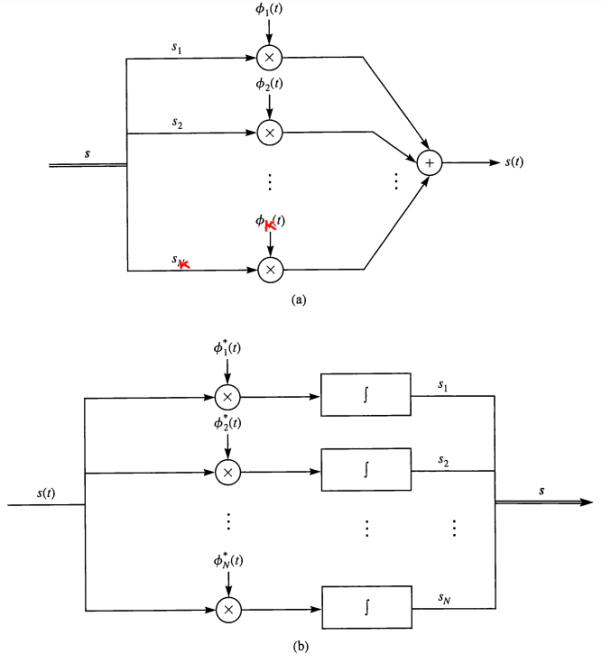
Fig 3. Vector to signal (a), and signal to vector (b) mappings

Q14) Explain geometric representation of signals?

A14)

Geometric representation of signals can provide a compact characterization of signals and can simplify analysis of their performance as modulation signals. Orthonormal bases are essential in geometry. Let {s1 (t), s2 (t), . . . , sM (t)} be a set of signals.

ψ1(t) = s1(t)/E1 where E1 =

s21 = < s2, ψ1 >=    and ψ2(t) = 1/2(s2(t) – s21(t) – s21ψ1)

2 =

ψk(t) = 1/2 ( sk(t) – )

k =

sm(t) =

The process continues until all of the M signals are exhausted. The results are N orthogonal signals with unit energy, {ψ1 (t), ψ2 (t), . . . , ψN (t)}. If the signals {s1 (t), . . . , sM (t)} are linearly independent, then N = M.

m ∈ {1, 2, . . . , M}

The M signals can be represented as

smn =< sm, ψn > and Em =

Q15) What are correlation receiver?

A15)

In other terms, the inner product is a correlation

But we want to build a receiver that does the minimum amount of calculation. If si(t) are non-orthogonal, then we can reduce the amount of correlation (and thus multiplication and addition) done in the receiver by instead, correlating with the basis functions, {φk(t)} N k=1. Correlation with the basis functions gives

x = [x1, x2, . . . , xN]T

Now that we’ve done these N correlations (inner products), we can compute the estimate of the received signal as

                                                       r(t) = bsi(t) + n(t)

                                                      n(t) = 0 and b = 1

                                                               x = ai

Where ai is the signal space vector for si(t).

Our signal set can be represented by the orthonormal basis functions, . Correlation with the basis functions gives

For k = 0 . . . K − 1. We denote vectors:

Hopefully, x and ai should be close since i was actually sent. In general, the pdf of x is multivariate Gaussian with each component xk independent, because

• xk = ai,k + nk
• ai,k is a deterministic constant
• The {nk} are i.i.d. Gaussian.

The joint pdf of x is

Q16) Explain in detail about matched filter receiver?

A16)

If a filter produces an output in such a way that it maximizes the ratio of output peak power to mean noise power in its frequency response, then that filter is called Matched filter.

Fig 4: Matched filter

Frequency Response Function of Matched Filter

The frequency response of the Matched filter will be proportional to the complex conjugate of the input signal’s spectrum. Mathematically, we can write the expression for frequency response function, H(f) of the Matched filter as −

H(f)=GaS∗(f)e−j2πft1    ………..1

Where,

Ga is the maximum gain of the Matched filter

S(f) is the Fourier transform of the input signal, s(t)

S∗(f) is the complex conjugate of S(f)

t1 is the time instant at which the signal observed to be maximum

In general, the value of Ga is considered as one. We will get the following equation by substituting Ga=1in Equation 1.

H(f)=S∗(f)e−j2πft1  ……..2

The frequency response function, H(f) of the Matched filter is having the magnitude of S∗(f)and phase angle of e−j2πft1, which varies uniformly with frequency.

Impulse Response of Matched Filter

In time domain, we will get the output, h(t) of Matched filter receiver by applying the inverse Fourier transform of the frequency response function, H(f).

h(t) =   .….3

Substitute, Equation 1 in Equation 3.

h(t) =

⇒ h(t) = ………4

We know the following relation.

S∗(f)=S(−f)                                   ……..5

Substitute, Equation 5 in Equation 4.

h(t) =

h(t) =

 h(t) = Gas(t1 – t)

In general, the value of Ga is considered as one. We will get the following equation by substituting Ga=1.

h(t)=s(t1−t)

The above equation proves that the impulse response of Matched filter is the mirror image of the received signal about a time instant t1. The following figures illustrate this concept.

Fig 5: Impulse response of Matched filter 

The received signal, s(t) and the impulse response, h(t) of the matched filter corresponding to the signal, s(t) are shown in the above figures.