Unit - 5
Frequency Domain analysis
Q1) Plot polar plot for T(S) = 1/S + 1
A1) (1) For polar plot substitute S=jw.
TF = 1/1 + jw
(2). Magnitude M = 1 + 0j / 1 + jw = 1/√1 + w2
(3). Phase φ = tan-1(0)/ tan-1w = - tan-1w
WMφ
0100
10.707-450
∞0-900
The plot is shown in fig. 1
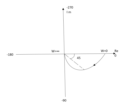
Fig 1 Polar Plot T(S) = 1/S + 1
Q2) Plot polar plot for T(S) = 1/(S+1)(S+2)
A2)
(1). S = jw
TF = 1/(1+jw)(2+jw)
(2). M = 1/(1+jw)(2+jw) = 1/-w2 + 3jw + 2
M = 1/√1 + w2√4 + w2
(3). Φ = - tan-1 w - tan-1(w/2)
WMΦ
00.500
10.316-71.560
20.158-108.430
∞0-1800
The plot is shown in fig 2

Fig 2 Polar Plot for T(S) = 1/(S+1)(S+2)
Intersection of polar plot with imaginary axis will be when real part of Transfer function = 0
M = 1/(jw + 1)(jw + 2)
= 1/-w2 + j3w + 2
Real part
Re(M) = 1/(2-w2)+j3w x (2-w2)-3jw/(2-w2)-3jw
Re(M) = (2-w2)/(2-w2+9w2) - 3jw/(2-w2) +9w2
Equating Real part = 0
(2-w2)/(2-w2)+ 9w2 = 0
W = +-√2
For w=√2 real part on the polar plot becomes zero.
So, polar plot intersects imaginary axis at w=√2 at φ = -900
Q3) Plot polar plot for T(S) = 1/(S+1)(S+2)(S+3)
A3)
(1). Substitute S =jw
(2). M = 1/√1+w2 √4+w2 √9+w2
(3). Φ = -tan-1w – tan-1 w/2 – tan-1w/3
WMφ
00.160
10.1-900
20.04-142.10
∞0-270
(4). Intersection of Polar plot with Real axis
M = 1/(S+1)(S+2)(S+3)
= 1/S3+6S2+11S+6
=1/(jw)2+6(jw)2+11jw+6
= 1/(6-6w2)+j(11w-w3)
Re(M) = 0 [Intersection with imaginary axis ]
M = 6-6w2/(6-6w2)2+(11w-w2)2 - j(11w-w3)/(6-6w2)2+(11w-w2)2
Re(M) = 0
6-6w2 = 0
w=1
Im(M) = 0[Intersection with Real axis]
11w = w3
The plot is shown in fig 3

Fig 3 Polar Plot for T(S) = 1/(S+1)(S+2)(S+3)
Q4) For T(S) = 1/S(S+1) plot polar plot?
A4)
(1). M = 1/W√1+w2
(2). Φ = -900 –
Tan -1(W/T)
WMφ
0∞-900
10.707-1350
20.45-153.40
∞0-1800
The plot is shown in fig.4

Fig 4 Polar Plot for T(S) = 1/S(S+1)
Q5) For T(s) = 1/S2(S+1) plot polar plot?
A5)
(1). M = 1/w2√1+jw
(2). Φ = -1800 – tan-1W/T
The plot is shown in fig. 5

Fig 5 Polar Plot for T(s) = 1/S2(S+1)
Q6) Sketch the bode plot for transfer function
G(S) = 
A6)
Replace S = j
G(j =
= 
This is type 0 system. So initial slope is 0 dB decade. The starting point is given as
20 log10 K = 20 log10 1000
= 60 dB
Corner frequency  1 =
1 =  = 10 rad/sec
 2 =
2 =  = 1000 rad/sec
Slope after  1 will be -20 dB/decade till second corner frequency i.e
  2 after
  2 the slope will be -40 dB/decade (-20+(-20)) as there are poles
For phase plot
 = tan-1 0.1
 - tan-1 0.001
For phase plot


100-900
200-9.450
300-104.80
400-110.360
500-115.420
600-120.00
700-124.170
800-127.940
900-131.350
1000 -134.420
The plot is shown in figure 6.

Fig 6. Magnitude Plot for G(S) = 
Q7) For the given transfer function determine
G(S) = 
Gain cross over frequency phase cross over frequency phase mergence and gain margin
A7)
Initial slope = 1
N = 1, (K)1/N = 2
K = 2
Corner frequency
 1 =
1 =  = 2 (slope -20 dB/decade
 2 =
2 =  = 20 (slope -40 dB/decade

Phase
 = tan-1
 - tan-1 0.5
  - tan-1 0.05
 = 900- tan-1 0.5
  - tan-1 0.05


1-119.430
5-172.230
10-195.250
15-209.270
20-219.30
25-226.760
30-232.490
35-236.980
40-240.570
45-243.490
50-245.910
Finding  gc (gain cross over frequency
M = 
4 =  2 (
2 ( (
(
 6 (6.25
 104) + 0.252
 4 +
4 + 2 = 4
2 = 4
Let  2 = x
2 = x
X3 (6.25 104) + 0.252
 2 + x = 4
X1 = 2.46
X2 = -399.9
X3 = -6.50
For x1 = 2.46
 gc = 3.99 rad/sec(from plot )
For phase margin
PM = 1800 - 
 = 900 – tan-1 (0.5×
 gc) – tan-1 (0.05 ×
  gc)
gc)
= -164.50
PM = 1800 - 164.50
= 15.50
For phase cross over frequency ( pc)
pc)
 = 900 – tan-1 (0.5
  ) – tan-1 (0.05
  )
)
-1800 = -900 – tan-1 (0.5  pc) – tan-1 (0.05
  pc)
pc)
-900 – tan-1 (0.5  pc) – tan-1 (0.05
  pc)
pc)
Taking than on both sides
Tan 900 = tan-1
Let tan-1 0.5  pc = A, tan-1 0.05
  pc = B
 = 00
= 00
 = 0
= 0
1 =0.5  pc 0.05
 pc
pc
 pc = 6.32 rad/sec
The plot is shown in figure 7.

Fig 7. Magnitude Plot for G(S) = 
Q8) For the given transfer function
G(S) = 
Plot the rode plot find PM and GM
A8)
T1 = 0.5  1 =
1 =  = 2 rad/sec
Zero so, slope (20 dB/decade)
T2 = 0.2  2 =
2 =  = 5 rad/sec
Pole, so slope (-20 dB/decade)
T3 = 0.1 = T4 = 0.1
 3 =
3 =  4 = 10 (2 pole ) (-40 db/decade)
1. Initial slope 0 dB/decade till  1 = 2 rad/sec
2. From  1 to
1 to 2 (i.e. 2 rad /sec to 5 rad/sec) slope will be 20 dB/decade
3. From  2 to
2 to  3 the slope will be 0 dB/decade (20 + (-20))
4. From  3 ,
3 , 4 the slope will be -40 dB/decade (0-20-20)
Phase plot
 = tan-1 0.5
 - tan-1 0.2
 - tan-1 0.1
 - tan-1 0.1


500-177.30
1000-178.60
1500-179.10
2000-179.40
2500-179.50
3000-179.530
3500-179.60
GM = 00
PM = 61.460
The plot is shown in figure 8.


Fig 8. Magnitude and Phase plot for G(S) = 
Q8) For the given transfer function plot the bode plot (magnitude plot)
G(S) = 
A9)
Given transfer function
G(S) = 
Converting above transfer function to standard from
G(S) = 
= 
1. As type 1 system, so initial slope will be -20 dB/decade
2. Final slope will be -60 dB/decade as order of system decides the final slope
3. Corner frequency
T1 =  ,
,  11= 5 (zero)
T2 = 1,  2 = 1 (pole)
4. Initial slope will cut zero dB axis at
(K)1/N = 10
i.e  = 10
= 10
5. Finding  n and
n and 
T(S) = 
T(S)= 
Comparing with standard second order system equation
S2+2 ns +
ns + n2
n2
 n = 11 rad/sec
 n = 5
n = 5
 11 = 5
 =
=  = 0.27
6. Maximum error
M = -20 log 2
= +6.5 dB
7. As K = 10, so whole plot will shift by 20 log 10 10 = 20 Db
The plot is shown in figure 9.
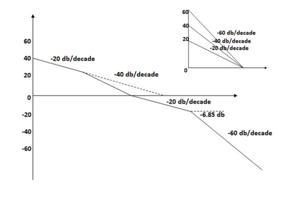
Fig 9. Magnitude plot for G(S) = 
Q10) For the given plot determine the transfer function

Fig 10 Magnitude plot for Q9
A10)
From figure 10, we can conclude that
1. Initial slope = -20 dB/decade so type -1
2. Initial slope alls 0 dB axis at  = 10 so
K1/N N = 1
(K)1/N = 10.
3. Corner frequency
 1 =
1 =  = 0.2 rad/sec
 2 =
2 =  = 0.125 rad/sec
4. At  = 5 the slope becomes -40 dB/decade, so there is a pole at
  = 5 as slope changes from -20 dB/decade to -40 dB/decade
5. At  = 8 the slope changes from -40 dB/decade to -20 dB/decade hence is a zero at
  = 8 (-40+(+20)=20)
6. Hence transfer function is
T(S) = 
Q9) For the transfer function below plot the Nyquist plot and also comment on stability? G(S) = 1/S+1
A11)
N = Z – P (No pole of right half of S plane P = 0)
P = 0, N = Z
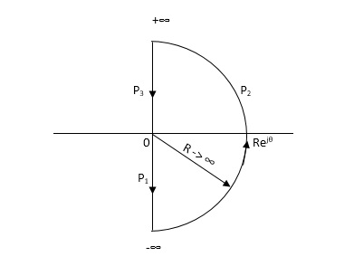
NYQUIST PATH:
P1 = W – (0 to - ∞)
P2 = ϴ( - π/2 to 0 to π/2 )
P3 = W(+∞ to 0)

Substituting S = jw
G(jw) = 1/jw + 1
M = 1/√1+W2
Φ = -tan-1(W/I)
For P1: W(0 to -∞)
WMφ
010
-11/√2+450
-∞0+900
Path P2:
W = Rejϴ R ∞ϴ -π/2 to 0 to π/2
G(jw) = 1/1+jw
= 1/1+j(Rejϴ) (neglecting 1 as R ∞)
M = 1/Rejϴ = 1/R e-jϴ
M = 0 e-jϴ = 0
Path P3:
W = -∞ to 0
M = 1/√1+W2, φ = -tan-1(W/I)
WMφ
∞0-900
11/√2-450
0100
The Nyquist Plot is shown in fig 11.

Fig 11. Nyquist plot for G(S) = 1/S+1
From plot we can see that -1 is not encircled so, N = 0
But N = Z, Z = 0
So, system is stable.
Q10) For the transfer function below plot the Nyquist Plot and comment on stability G(S) = 1/(S + 4)(S + 5)
A12)
N = Z – P, P = 0, No pole on right half of S-plane
N = Z
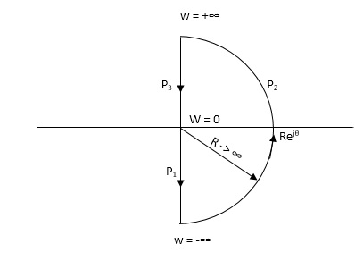
NYQUIST PATH
P1 = W(0 to -∞)
P2 = ϴ(-π/2 to 0 to +π/2)
P3 = W(∞ to 0)

Path P1 W(0 to -∞)
M = 1/√42 + w2 √52 + w2
Φ = -tan-1(W/4) – tan-1(W/5)
WMΦ
01/2000
-10.04725.350
-∞0+1800
Path P3 will be the mirror image across the real axis.
Path P2: ϴ(-π/2 to 0 to +π/2)
S = Rejϴ
G(S) = 1/(Rejϴ + 4)( Rejϴ + 5)
R∞
= 1/ R2e2jϴ = 0.e-j2ϴ = 0
The plot is shown in fig 12. From plot N=0, Z=0, system stable.

Fig 12. Nyquist plot for G(S) = 1/(S + 4)(S + 5)
Q11) For the given transfer function, plot the Nyquist plot and comment on stability G(S) = k/S2(S + 10)?
A13)
As the poles exists at origin. So, first time we do not include poles in Nyquist plot. Then check the stability for second case we include the poles at origin in Nyquist path. Then again check the stability.
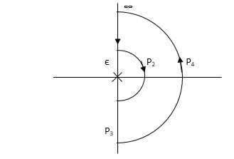
PART – 1: Not including poles at origin in the Nyquist Path.

P1 W(∞ Ɛ) where Ɛ 0
P2 S = Ɛejϴϴ(+π/2 to 0 to -π/2)
P3 W = -Ɛ to -∞
P4 S = Rejϴ, R ∞, ϴ = -π/2 to 0 to +π/2
For P1
M = 1/w.w√102 + w2 = 1/w2√102 + w2
Φ = -1800 – tan-1(w/10)
WMΦ
∞0-3 π/2
Ɛ∞-1800
Path P3 will be mirror image of P1 about Real axis.
G(Ɛ ejϴ) = 1/( Ɛ ejϴ)2(Ɛ ejϴ + 10)
Ɛ 0, ϴ = π/2 to 0 to -π/2
= 1/ Ɛ2 e2jϴ(Ɛ ejϴ + 10)
= ∞.e-j2ϴ [ -2ϴ = -π to 0 to +π ]
Path P2 will be formed by rotating through -π to 0 to +π
Path P4 S = Rejϴ R ∞ ϴ = -π/2 to 0 to +π/2
G(Rejϴ) = 1/ (Rejϴ)2(10 + Rejϴ)
= 0
N = Z – P
No poles on right half of S plane so, P = 0
N = Z – 0
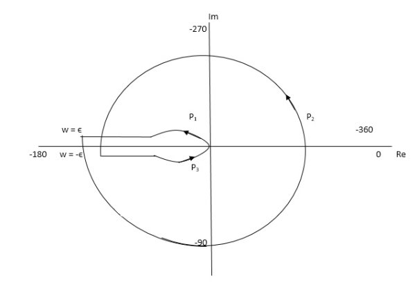
Fig 13. Nyquist plot for G(S) = k/S2(S + 10)
But from plot shown in fig 13. It is clear that number of encirclements in Anticlockwise direction. So,
N = 2
N = Z – P
2 = Z – 0
Z = 2
Hence, system unstable.
PART 2 Including poles at origin in the Nyquist Path.
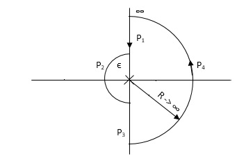
P1 W(∞ to Ɛ) Ɛ 0
P2 S = ƐejϴƐ 0 ϴ(+π/2 to +π to +3π/2)
P3 W(-Ɛ to -∞) Ɛ 0
P4 S = Rejϴ, R ∞, ϴ(3π/2 to 2π to +5π/2)
M = 1/W2√102 + W2 , φ = - π – tan-1(W/10)
P1W(∞ to Ɛ)
WMφ
∞0-3 π/2
Ɛ∞-1800
P3( mirror image of P1)
P2S = Ɛejϴ
G(Ɛejϴ) = 1/ Ɛ2e2jϴ(10 + Ɛejϴ)
Ɛ 0
G(Ɛejϴ) = 1/ Ɛ2e2jϴ(10)
= ∞. e-j2ϴϴ(π/2 to π to 3π/2)
-2ϴ = (-π to -2π to -3π)
P4 = 0

Fig 14. Nyquist Plot for G(S) = k/S2(S + 10)
The plot is shown in fig. From the plot it is clear that there is no encirclement of -1 in Nyquist path. (N = 0). But the two poles at origin lies to the right half of S-plane in Nyquist path.(P = 2)[see path P2]
N = Z – P
0 = Z – 2
Z = 2
Hence, system is unstable.
Path P2 will be formed by rotating through -π to -2π to -3π
Q12) Explain relation between time and frequency response?
A14) The calculation of system parameters for higher order systems is difficult in time domain analysis. This can be overcome by frequency domain analysis. As the frequency response of a linear time invariant system is independent of amplitude and phase of the input test signal. The effect of noise and parameter variation in frequency domain can be easily computed.
In frequency response can be determine by calculating the phase and amplitude oof the given system transfer function. If a sinusoidal signal XG(j )sin
)sin t then its amplitude will be
C(t) = XG(j )sin
)sin t
t
= X|G(j )|
)| sin
sin t
t
Magnitude = |G(j )|
)|
Phase = 
In polar form = |G(j )|
)|
The transfer function of second order system is shown as
C(S)/R(S) = W2n / S2 + 2ξWnS + W2n - - (1)
ξ = Ramping factor
Wn = Undamped natural frequency for frequency response let S = jw
C(jw) / R(jw) = W2n / (jw)2 + 2 ξWn(jw) + W2n
Let U = W/Wn above equation becomes
T(jw) = W2n / 1 – U2 + j2 ξU
So,
| T(jw) | = M = 1/√(1 – u2)2 + (2ξU)2 - - (2)
T(jw) = φ = -tan-1[ 2ξu/(1-u2)] - - (3)
For sinusoidal input the output response for the system is given by
C(t) = 1/√(1-u2)2 + (2ξu)2Sin[wt - tan-1 2ξu/1-u2] - - (4)
The frequency where M has the peak value is known as Resonant frequency Wn. This frequency is given as (from eqn (2)).
DM/du|u=ur = Wr = Wn√(1-2ξ2) - - (5)
From equation(2) the maximum value of magnitude is known as Resonant peak.
Mr = 1/2ξ√1-ξ2 - - (6)
The phase angle at resonant frequency is given as
Φr = - tan-1 [√1-2ξ2/ ξ] - - (7)
As we already know for step response of second order system the value of damped frequency and peak overshoot are given as
Wd = Wn√1-ξ2 - - (8)
Mp = e- πξ2|√1-ξ2 - - (9)

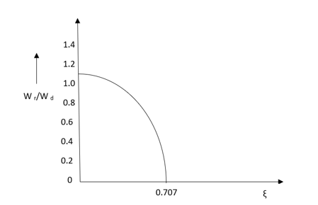
Fig 15. Frequency Domain Specification
The comparison of Mr and Mp is shown in figure. The two performance indices are correlated as both are functions of the damping factor ξ only. When subjected to step input the system with given value of Mr of its frequency response will exhibit a corresponding value of Mp.
Similarly the correlation of Wr and Wd is shown in figure for the given input step response [ from eqn(5) & eqn(8) ]
Wr/Wd = √(1- 2ξ2)/(1-ξ2)
Mp = Peak overshoot of step response
Mr = Resonant Peak of frequency response
Wr = Resonant frequency of Frequency response
Wd = Damping frequency of oscillation of step response.
From fig(17) it is clear that for ξ> 1/2, value of Mr does not exists.
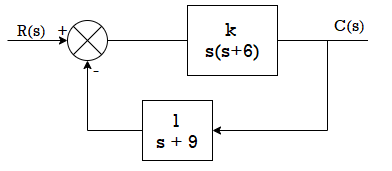
Q13) For the following system shown below find the phase margin and gain margin if the value of k=500 by using Nyquist plot.
A15)
G(s)H(s) = 500/s(s+6)(s+9)
The polar plot for above OLTF is shown in figure below.
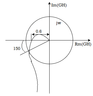
Fig 16. Polar Plot for given system
From figure we see A=0.6,
The GM in dB = -20logA.
= 4.43dB
PM = 1800-1650
= 150
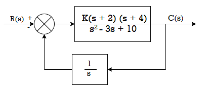
Q14) For the system shown in figure, find the GM and PM using Nyquist plot for k=10. Find also range of k for stability?

A16)
The transfer function is G(s) H(s) = 10(s+2(s+4)/s(s2 – 3s+10)
As the OLTF is unstable system so PM and GM concepts cannot be applied.
G(jω) H(jω) = 10(jω+2) (jω+4)/ jω(-ω2 -3 jω+10)
| G(jω) H(jω)|= 10(√4+ω2)( √16+ω2)/ ω√[(10-ω)2+9 ω2]
 G(jω)H(jω) = -900 +tan-1(ω/2) + tan-1(ω/4) - tan-1 (-3ω/10- ω2)
The polar plot for above system is shown below.

Fig 17. Polar plot for the given system
From figure we have A=2.6 and ɸ =-1350
The GM in dB = -20logA.
= -8.3dB
As GM is negative it indicates that system is open loop unstable.
PM = 1800-1650 = 450
Q15) Write short note on Nicholas chart?
A17)
The Nichols plot is named after the American engineer N.B Nichols who formulated this plot. Compensators can be designed using Nichols plot. Nichols plot technique is however also used in designing of dc motor. This is used in signal processing and control design. Nyquist plot in complex plane shows how phase of transfer function and frequency variation of magnitude are related. • Angle of positive real axis determines the phase and distance from origin of complex plane determines the gain.
Advantages
- Gain and phase margin can be determined easily and also graphically.
- Closed loop frequency response is obtained from open loop frequency response.
- Gain of the system can be adjusted to suitable values.
- Nichols chart provides frequency domain specifications.
Disadvantage
Using Nichols plot small changes in gain cannot be encountered easily.
Q16) What are M circles? Derive its equation for forming circle?
A18)
Constant magnitude loci that are M-circles and constant phase angle loci that are N-circles are the fundamental components. The constant M and constant N circles in G (jω) plane can be used for the analysis and design of control systems. However, the constant M and constant N circles in gain phase plane are prepared for system design and analysis as these plots supply information with fewer manipulations. Gain phase plane is the graph having gain in decibel along the ordinate (vertical axis) and phase angle along the abscissa (horizontal axis).
For Constant M Circle
For a system with unity feedback having transfer function
T(s)= G(s)/1+G(s)
Replace s=jω
T(jω) = G(jω)/1+G(jω)
But we can write G(jω)= X(jω)+jY(jω)
The closed loop transfer function T(s) is
T(jω) = X+jY/1+X+jY= Mejα
M= |X+jY|/|1+X+jY|
M2=X2+Y2/(1+X2) + Y2
Solving above equation we get
[X-(M2/1-M2)]2 + Y2 = ([M/1-M2)]2
This is equation of circle with centre (M2/1-M2),0 and radius M/1-M2
When M<1, M decreases the radius of the circle decreases and centres located on positive real axis shifts towards origin. When M=0 the radius becomes 0 and the centre (0,0). This is shown in figure above.
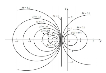
Fig 18. Constant M circle
Q17) For T(S) = 1/S plot polar plot?
A19)
(1). S = jw
(2). M = 1/W
(3). Φ = -tan-1(W/O) = -900
WMφ
0∞-900
11-900
20.5-900
∞0-900
The plot is shown in fig. 19.

Fig 19. Polar plot for T(S) = 1/S
Q18) Define the relationship between time and frequency response?
A20)
The calculation of system parameters for higher order systems is difficult in time domain analysis. This can be overcome by frequency domain analysis. As the frequency response of a linear time invariant system is independent of amplitude and phase of the input test signal. The effect of noise and parameter variation in frequency domain can be easily computed.
In frequency response can be determine by calculating the phase and amplitude oof the given system transfer function. If a sinusoidal signal XG(j )sin
)sin t then its amplitude will be
C(t) = XG(j )sin
)sin t
t
= X|G(j )|
)| sin
sin t
t
Magnitude = |G(j )|
)|
Phase = 
In polar form = |G(j )|
)|
The transfer function of second order system is shown as
C(S)/R(S) = W2n / S2 + 2ξWnS + W2n - - (1)
ξ = Ramping factor
Wn = Undamped natural frequency for frequency response let S = jw
C(jw) / R(jw) = W2n / (jw)2 + 2 ξWn(jw) + W2n
Let U = W/Wn above equation becomes
T(jw) = W2n / 1 – U2 + j2 ξU
So,
| T(jw) | = M = 1/√(1 – u2)2 + (2ξU)2 - - (2)
T(jw) = φ = -tan-1[ 2ξu/(1-u2)] - - (3)
For sinusoidal input the output response for the system is given by
C(t) = 1/√(1-u2)2 + (2ξu)2Sin[wt - tan-1 2ξu/1-u2] - - (4)
The frequency where M has the peak value is known as Resonant frequency Wn. This frequency is given as (from eqn (2)).
DM/du|u=ur = Wr = Wn√(1-2ξ2) - - (5)
From equation(2) the maximum value of magnitude is known as Resonant peak.
Mr = 1/2ξ√1-ξ2 - - (6)
The phase angle at resonant frequency is given as
Φr = - tan-1 [√1-2ξ2/ ξ] - - (7)
As we already know for step response of second order system the value of damped frequency and peak overshoot are given as
Wd = Wn√1-ξ2 - - (8)
Mp = e- πξ2|√1-ξ2 - - (9)
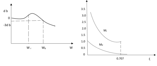

Fig 20. Frequency Domain Specification
The comparison of Mr and Mp is shown in figure. The two performance indices are correlated as both are functions of the damping factor ξ only. When subjected to step input the system with given value of Mr of its frequency response will exhibit a corresponding value of Mp.
Similarly the correlation of Wr and Wd is shown in figure for the given input step response [ from eqn(5) & eqn(8) ]
Wr/Wd = √(1- 2ξ2)/(1-ξ2)
Mp = Peak overshoot of step response
Mr = Resonant Peak of frequency response
Wr = Resonant frequency of Frequency response
Wd = Damping frequency of oscillation of step response.
From fig(1) it is clear that for ξ> 1/2, value of Mr does not exists.
Unit - 5
Frequency Domain analysis
Q1) Plot polar plot for T(S) = 1/S + 1
A1) (1) For polar plot substitute S=jw.
TF = 1/1 + jw
(2). Magnitude M = 1 + 0j / 1 + jw = 1/√1 + w2
(3). Phase φ = tan-1(0)/ tan-1w = - tan-1w
WMφ
0100
10.707-450
∞0-900
The plot is shown in fig. 1

Fig 1 Polar Plot T(S) = 1/S + 1
Q2) Plot polar plot for T(S) = 1/(S+1)(S+2)
A2)
(1). S = jw
TF = 1/(1+jw)(2+jw)
(2). M = 1/(1+jw)(2+jw) = 1/-w2 + 3jw + 2
M = 1/√1 + w2√4 + w2
(3). Φ = - tan-1 w - tan-1(w/2)
WMΦ
00.500
10.316-71.560
20.158-108.430
∞0-1800
The plot is shown in fig 2

Fig 2 Polar Plot for T(S) = 1/(S+1)(S+2)
Intersection of polar plot with imaginary axis will be when real part of Transfer function = 0
M = 1/(jw + 1)(jw + 2)
= 1/-w2 + j3w + 2
Real part
Re(M) = 1/(2-w2)+j3w x (2-w2)-3jw/(2-w2)-3jw
Re(M) = (2-w2)/(2-w2+9w2) - 3jw/(2-w2) +9w2
Equating Real part = 0
(2-w2)/(2-w2)+ 9w2 = 0
W = +-√2
For w=√2 real part on the polar plot becomes zero.
So, polar plot intersects imaginary axis at w=√2 at φ = -900
Q3) Plot polar plot for T(S) = 1/(S+1)(S+2)(S+3)
A3)
(1). Substitute S =jw
(2). M = 1/√1+w2 √4+w2 √9+w2
(3). Φ = -tan-1w – tan-1 w/2 – tan-1w/3
WMφ
00.160
10.1-900
20.04-142.10
∞0-270
(4). Intersection of Polar plot with Real axis
M = 1/(S+1)(S+2)(S+3)
= 1/S3+6S2+11S+6
=1/(jw)2+6(jw)2+11jw+6
= 1/(6-6w2)+j(11w-w3)
Re(M) = 0 [Intersection with imaginary axis ]
M = 6-6w2/(6-6w2)2+(11w-w2)2 - j(11w-w3)/(6-6w2)2+(11w-w2)2
Re(M) = 0
6-6w2 = 0
w=1
Im(M) = 0[Intersection with Real axis]
11w = w3
The plot is shown in fig 3
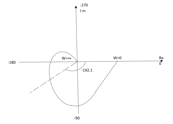
Fig 3 Polar Plot for T(S) = 1/(S+1)(S+2)(S+3)
Q4) For T(S) = 1/S(S+1) plot polar plot?
A4)
(1). M = 1/W√1+w2
(2). Φ = -900 –
Tan -1(W/T)
WMφ
0∞-900
10.707-1350
20.45-153.40
∞0-1800
The plot is shown in fig.4
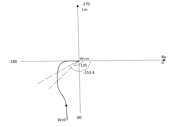
Fig 4 Polar Plot for T(S) = 1/S(S+1)
Q5) For T(s) = 1/S2(S+1) plot polar plot?
A5)
(1). M = 1/w2√1+jw
(2). Φ = -1800 – tan-1W/T
The plot is shown in fig. 5
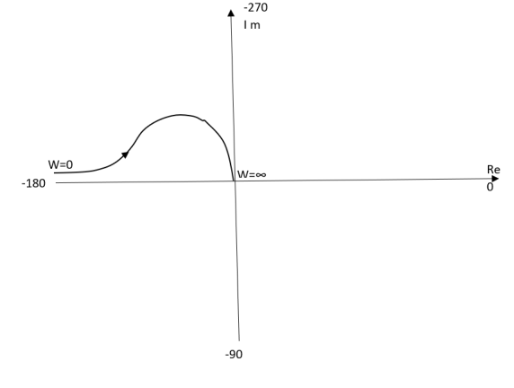
Fig 5 Polar Plot for T(s) = 1/S2(S+1)
Q6) Sketch the bode plot for transfer function
G(S) = 
A6)
Replace S = j
G(j =
= 
This is type 0 system. So initial slope is 0 dB decade. The starting point is given as
20 log10 K = 20 log10 1000
= 60 dB
Corner frequency  1 =
1 =  = 10 rad/sec
 2 =
2 =  = 1000 rad/sec
Slope after  1 will be -20 dB/decade till second corner frequency i.e
  2 after
  2 the slope will be -40 dB/decade (-20+(-20)) as there are poles
For phase plot
 = tan-1 0.1
 - tan-1 0.001
For phase plot


100-900
200-9.450
300-104.80
400-110.360
500-115.420
600-120.00
700-124.170
800-127.940
900-131.350
1000 -134.420
The plot is shown in figure 6.

Fig 6. Magnitude Plot for G(S) = 
Q7) For the given transfer function determine
G(S) = 
Gain cross over frequency phase cross over frequency phase mergence and gain margin
A7)
Initial slope = 1
N = 1, (K)1/N = 2
K = 2
Corner frequency
 1 =
1 =  = 2 (slope -20 dB/decade
 2 =
2 =  = 20 (slope -40 dB/decade

Phase
 = tan-1
 - tan-1 0.5
  - tan-1 0.05
 = 900- tan-1 0.5
  - tan-1 0.05


1-119.430
5-172.230
10-195.250
15-209.270
20-219.30
25-226.760
30-232.490
35-236.980
40-240.570
45-243.490
50-245.910
Finding  gc (gain cross over frequency
M = 
4 =  2 (
2 ( (
(
 6 (6.25
 104) + 0.252
 4 +
4 + 2 = 4
2 = 4
Let  2 = x
2 = x
X3 (6.25 104) + 0.252
 2 + x = 4
X1 = 2.46
X2 = -399.9
X3 = -6.50
For x1 = 2.46
 gc = 3.99 rad/sec(from plot )
For phase margin
PM = 1800 - 
 = 900 – tan-1 (0.5×
 gc) – tan-1 (0.05 ×
  gc)
gc)
= -164.50
PM = 1800 - 164.50
= 15.50
For phase cross over frequency ( pc)
pc)
 = 900 – tan-1 (0.5
  ) – tan-1 (0.05
  )
)
-1800 = -900 – tan-1 (0.5  pc) – tan-1 (0.05
  pc)
pc)
-900 – tan-1 (0.5  pc) – tan-1 (0.05
  pc)
pc)
Taking than on both sides
Tan 900 = tan-1
Let tan-1 0.5  pc = A, tan-1 0.05
  pc = B
 = 00
= 00
 = 0
= 0
1 =0.5  pc 0.05
 pc
pc
 pc = 6.32 rad/sec
The plot is shown in figure 7.
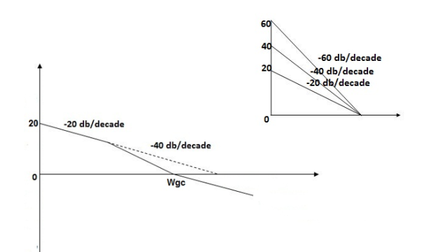
Fig 7. Magnitude Plot for G(S) = 
Q8) For the given transfer function
G(S) = 
Plot the rode plot find PM and GM
A8)
T1 = 0.5  1 =
1 =  = 2 rad/sec
Zero so, slope (20 dB/decade)
T2 = 0.2  2 =
2 =  = 5 rad/sec
Pole, so slope (-20 dB/decade)
T3 = 0.1 = T4 = 0.1
 3 =
3 =  4 = 10 (2 pole ) (-40 db/decade)
1. Initial slope 0 dB/decade till  1 = 2 rad/sec
2. From  1 to
1 to 2 (i.e. 2 rad /sec to 5 rad/sec) slope will be 20 dB/decade
3. From  2 to
2 to  3 the slope will be 0 dB/decade (20 + (-20))
4. From  3 ,
3 , 4 the slope will be -40 dB/decade (0-20-20)
Phase plot
 = tan-1 0.5
 - tan-1 0.2
 - tan-1 0.1
 - tan-1 0.1


500-177.30
1000-178.60
1500-179.10
2000-179.40
2500-179.50
3000-179.530
3500-179.60
GM = 00
PM = 61.460
The plot is shown in figure 8.
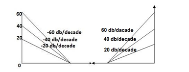
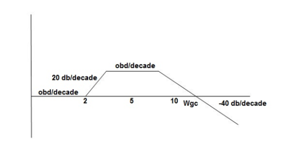

Fig 8. Magnitude and Phase plot for G(S) = 
Q8) For the given transfer function plot the bode plot (magnitude plot)
G(S) = 
A9)
Given transfer function
G(S) = 
Converting above transfer function to standard from
G(S) = 
= 
1. As type 1 system, so initial slope will be -20 dB/decade
2. Final slope will be -60 dB/decade as order of system decides the final slope
3. Corner frequency
T1 =  ,
,  11= 5 (zero)
T2 = 1,  2 = 1 (pole)
4. Initial slope will cut zero dB axis at
(K)1/N = 10
i.e  = 10
= 10
5. Finding  n and
n and 
T(S) = 
T(S)= 
Comparing with standard second order system equation
S2+2 ns +
ns + n2
n2
 n = 11 rad/sec
 n = 5
n = 5
 11 = 5
 =
=  = 0.27
6. Maximum error
M = -20 log 2
= +6.5 dB
7. As K = 10, so whole plot will shift by 20 log 10 10 = 20 Db
The plot is shown in figure 9.

Fig 9. Magnitude plot for G(S) = 
Q10) For the given plot determine the transfer function

Fig 10 Magnitude plot for Q9
A10)
From figure 10, we can conclude that
1. Initial slope = -20 dB/decade so type -1
2. Initial slope alls 0 dB axis at  = 10 so
K1/N N = 1
(K)1/N = 10.
3. Corner frequency
 1 =
1 =  = 0.2 rad/sec
 2 =
2 =  = 0.125 rad/sec
4. At  = 5 the slope becomes -40 dB/decade, so there is a pole at
  = 5 as slope changes from -20 dB/decade to -40 dB/decade
5. At  = 8 the slope changes from -40 dB/decade to -20 dB/decade hence is a zero at
  = 8 (-40+(+20)=20)
6. Hence transfer function is
T(S) = 
Q9) For the transfer function below plot the Nyquist plot and also comment on stability? G(S) = 1/S+1
A11)
N = Z – P (No pole of right half of S plane P = 0)
P = 0, N = Z
NYQUIST PATH:
P1 = W – (0 to - ∞)
P2 = ϴ( - π/2 to 0 to π/2 )
P3 = W(+∞ to 0)

Substituting S = jw
G(jw) = 1/jw + 1
M = 1/√1+W2
Φ = -tan-1(W/I)
For P1: W(0 to -∞)
WMφ
010
-11/√2+450
-∞0+900
Path P2:
W = Rejϴ R ∞ϴ -π/2 to 0 to π/2
G(jw) = 1/1+jw
= 1/1+j(Rejϴ) (neglecting 1 as R ∞)
M = 1/Rejϴ = 1/R e-jϴ
M = 0 e-jϴ = 0
Path P3:
W = -∞ to 0
M = 1/√1+W2, φ = -tan-1(W/I)
WMφ
∞0-900
11/√2-450
0100
The Nyquist Plot is shown in fig 11.

Fig 11. Nyquist plot for G(S) = 1/S+1
From plot we can see that -1 is not encircled so, N = 0
But N = Z, Z = 0
So, system is stable.
Q10) For the transfer function below plot the Nyquist Plot and comment on stability G(S) = 1/(S + 4)(S + 5)
A12)
N = Z – P, P = 0, No pole on right half of S-plane
N = Z
NYQUIST PATH
P1 = W(0 to -∞)
P2 = ϴ(-π/2 to 0 to +π/2)
P3 = W(∞ to 0)

Path P1 W(0 to -∞)
M = 1/√42 + w2 √52 + w2
Φ = -tan-1(W/4) – tan-1(W/5)
WMΦ
01/2000
-10.04725.350
-∞0+1800
Path P3 will be the mirror image across the real axis.
Path P2: ϴ(-π/2 to 0 to +π/2)
S = Rejϴ
G(S) = 1/(Rejϴ + 4)( Rejϴ + 5)
R∞
= 1/ R2e2jϴ = 0.e-j2ϴ = 0
The plot is shown in fig 12. From plot N=0, Z=0, system stable.

Fig 12. Nyquist plot for G(S) = 1/(S + 4)(S + 5)
Q11) For the given transfer function, plot the Nyquist plot and comment on stability G(S) = k/S2(S + 10)?
A13)
As the poles exists at origin. So, first time we do not include poles in Nyquist plot. Then check the stability for second case we include the poles at origin in Nyquist path. Then again check the stability.
PART – 1: Not including poles at origin in the Nyquist Path.
P1 W(∞ Ɛ) where Ɛ 0
P2 S = Ɛejϴϴ(+π/2 to 0 to -π/2)
P3 W = -Ɛ to -∞
P4 S = Rejϴ, R ∞, ϴ = -π/2 to 0 to +π/2
For P1
M = 1/w.w√102 + w2 = 1/w2√102 + w2
Φ = -1800 – tan-1(w/10)
WMΦ
∞0-3 π/2
Ɛ∞-1800
Path P3 will be mirror image of P1 about Real axis.
G(Ɛ ejϴ) = 1/( Ɛ ejϴ)2(Ɛ ejϴ + 10)
Ɛ 0, ϴ = π/2 to 0 to -π/2
= 1/ Ɛ2 e2jϴ(Ɛ ejϴ + 10)
= ∞.e-j2ϴ [ -2ϴ = -π to 0 to +π ]
Path P2 will be formed by rotating through -π to 0 to +π
Path P4 S = Rejϴ R ∞ ϴ = -π/2 to 0 to +π/2
G(Rejϴ) = 1/ (Rejϴ)2(10 + Rejϴ)
= 0
N = Z – P
No poles on right half of S plane so, P = 0
N = Z – 0

Fig 13. Nyquist plot for G(S) = k/S2(S + 10)
But from plot shown in fig 13. It is clear that number of encirclements in Anticlockwise direction. So,
N = 2
N = Z – P
2 = Z – 0
Z = 2
Hence, system unstable.
PART 2 Including poles at origin in the Nyquist Path.

P1 W(∞ to Ɛ) Ɛ 0
P2 S = ƐejϴƐ 0 ϴ(+π/2 to +π to +3π/2)
P3 W(-Ɛ to -∞) Ɛ 0
P4 S = Rejϴ, R ∞, ϴ(3π/2 to 2π to +5π/2)
M = 1/W2√102 + W2 , φ = - π – tan-1(W/10)
P1W(∞ to Ɛ)
WMφ
∞0-3 π/2
Ɛ∞-1800
P3( mirror image of P1)
P2S = Ɛejϴ
G(Ɛejϴ) = 1/ Ɛ2e2jϴ(10 + Ɛejϴ)
Ɛ 0
G(Ɛejϴ) = 1/ Ɛ2e2jϴ(10)
= ∞. e-j2ϴϴ(π/2 to π to 3π/2)
-2ϴ = (-π to -2π to -3π)
P4 = 0

Fig 14. Nyquist Plot for G(S) = k/S2(S + 10)
The plot is shown in fig. From the plot it is clear that there is no encirclement of -1 in Nyquist path. (N = 0). But the two poles at origin lies to the right half of S-plane in Nyquist path.(P = 2)[see path P2]
N = Z – P
0 = Z – 2
Z = 2
Hence, system is unstable.
Path P2 will be formed by rotating through -π to -2π to -3π
Q12) Explain relation between time and frequency response?
A14) The calculation of system parameters for higher order systems is difficult in time domain analysis. This can be overcome by frequency domain analysis. As the frequency response of a linear time invariant system is independent of amplitude and phase of the input test signal. The effect of noise and parameter variation in frequency domain can be easily computed.
In frequency response can be determine by calculating the phase and amplitude oof the given system transfer function. If a sinusoidal signal XG(j )sin
)sin t then its amplitude will be
C(t) = XG(j )sin
)sin t
t
= X|G(j )|
)| sin
sin t
t
Magnitude = |G(j )|
)|
Phase = 
In polar form = |G(j )|
)|
The transfer function of second order system is shown as
C(S)/R(S) = W2n / S2 + 2ξWnS + W2n - - (1)
ξ = Ramping factor
Wn = Undamped natural frequency for frequency response let S = jw
C(jw) / R(jw) = W2n / (jw)2 + 2 ξWn(jw) + W2n
Let U = W/Wn above equation becomes
T(jw) = W2n / 1 – U2 + j2 ξU
So,
| T(jw) | = M = 1/√(1 – u2)2 + (2ξU)2 - - (2)
T(jw) = φ = -tan-1[ 2ξu/(1-u2)] - - (3)
For sinusoidal input the output response for the system is given by
C(t) = 1/√(1-u2)2 + (2ξu)2Sin[wt - tan-1 2ξu/1-u2] - - (4)
The frequency where M has the peak value is known as Resonant frequency Wn. This frequency is given as (from eqn (2)).
DM/du|u=ur = Wr = Wn√(1-2ξ2) - - (5)
From equation(2) the maximum value of magnitude is known as Resonant peak.
Mr = 1/2ξ√1-ξ2 - - (6)
The phase angle at resonant frequency is given as
Φr = - tan-1 [√1-2ξ2/ ξ] - - (7)
As we already know for step response of second order system the value of damped frequency and peak overshoot are given as
Wd = Wn√1-ξ2 - - (8)
Mp = e- πξ2|√1-ξ2 - - (9)
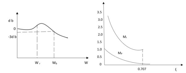

Fig 15. Frequency Domain Specification
The comparison of Mr and Mp is shown in figure. The two performance indices are correlated as both are functions of the damping factor ξ only. When subjected to step input the system with given value of Mr of its frequency response will exhibit a corresponding value of Mp.
Similarly the correlation of Wr and Wd is shown in figure for the given input step response [ from eqn(5) & eqn(8) ]
Wr/Wd = √(1- 2ξ2)/(1-ξ2)
Mp = Peak overshoot of step response
Mr = Resonant Peak of frequency response
Wr = Resonant frequency of Frequency response
Wd = Damping frequency of oscillation of step response.
From fig(17) it is clear that for ξ> 1/2, value of Mr does not exists.
Q13) For the following system shown below find the phase margin and gain margin if the value of k=500 by using Nyquist plot.

A15)
G(s)H(s) = 500/s(s+6)(s+9)
The polar plot for above OLTF is shown in figure below.

Fig 16. Polar Plot for given system
From figure we see A=0.6,
The GM in dB = -20logA.
= 4.43dB
PM = 1800-1650
= 150
Q14) For the system shown in figure, find the GM and PM using Nyquist plot for k=10. Find also range of k for stability?
A16)
The transfer function is G(s) H(s) = 10(s+2(s+4)/s(s2 – 3s+10)
As the OLTF is unstable system so PM and GM concepts cannot be applied.
G(jω) H(jω) = 10(jω+2) (jω+4)/ jω(-ω2 -3 jω+10)
| G(jω) H(jω)|= 10(√4+ω2)( √16+ω2)/ ω√[(10-ω)2+9 ω2]
 G(jω)H(jω) = -900 +tan-1(ω/2) + tan-1(ω/4) - tan-1 (-3ω/10- ω2)
The polar plot for above system is shown below.

Fig 17. Polar plot for the given system
From figure we have A=2.6 and ɸ =-1350
The GM in dB = -20logA.
= -8.3dB
As GM is negative it indicates that system is open loop unstable.
PM = 1800-1650 = 450
Q15) Write short note on Nicholas chart?
A17)
The Nichols plot is named after the American engineer N.B Nichols who formulated this plot. Compensators can be designed using Nichols plot. Nichols plot technique is however also used in designing of dc motor. This is used in signal processing and control design. Nyquist plot in complex plane shows how phase of transfer function and frequency variation of magnitude are related. • Angle of positive real axis determines the phase and distance from origin of complex plane determines the gain.
Advantages
- Gain and phase margin can be determined easily and also graphically.
- Closed loop frequency response is obtained from open loop frequency response.
- Gain of the system can be adjusted to suitable values.
- Nichols chart provides frequency domain specifications.
Disadvantage
Using Nichols plot small changes in gain cannot be encountered easily.
Q16) What are M circles? Derive its equation for forming circle?
A18)
Constant magnitude loci that are M-circles and constant phase angle loci that are N-circles are the fundamental components. The constant M and constant N circles in G (jω) plane can be used for the analysis and design of control systems. However, the constant M and constant N circles in gain phase plane are prepared for system design and analysis as these plots supply information with fewer manipulations. Gain phase plane is the graph having gain in decibel along the ordinate (vertical axis) and phase angle along the abscissa (horizontal axis).
For Constant M Circle
For a system with unity feedback having transfer function
T(s)= G(s)/1+G(s)
Replace s=jω
T(jω) = G(jω)/1+G(jω)
But we can write G(jω)= X(jω)+jY(jω)
The closed loop transfer function T(s) is
T(jω) = X+jY/1+X+jY= Mejα
M= |X+jY|/|1+X+jY|
M2=X2+Y2/(1+X2) + Y2
Solving above equation we get
[X-(M2/1-M2)]2 + Y2 = ([M/1-M2)]2
This is equation of circle with centre (M2/1-M2),0 and radius M/1-M2
When M<1, M decreases the radius of the circle decreases and centres located on positive real axis shifts towards origin. When M=0 the radius becomes 0 and the centre (0,0). This is shown in figure above.

Fig 18. Constant M circle
Q17) For T(S) = 1/S plot polar plot?
A19)
(1). S = jw
(2). M = 1/W
(3). Φ = -tan-1(W/O) = -900
WMφ
0∞-900
11-900
20.5-900
∞0-900
The plot is shown in fig. 19.
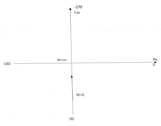
Fig 19. Polar plot for T(S) = 1/S
Q18) Define the relationship between time and frequency response?
A20)
The calculation of system parameters for higher order systems is difficult in time domain analysis. This can be overcome by frequency domain analysis. As the frequency response of a linear time invariant system is independent of amplitude and phase of the input test signal. The effect of noise and parameter variation in frequency domain can be easily computed.
In frequency response can be determine by calculating the phase and amplitude oof the given system transfer function. If a sinusoidal signal XG(j )sin
)sin t then its amplitude will be
C(t) = XG(j )sin
)sin t
t
= X|G(j )|
)| sin
sin t
t
Magnitude = |G(j )|
)|
Phase = 
In polar form = |G(j )|
)|
The transfer function of second order system is shown as
C(S)/R(S) = W2n / S2 + 2ξWnS + W2n - - (1)
ξ = Ramping factor
Wn = Undamped natural frequency for frequency response let S = jw
C(jw) / R(jw) = W2n / (jw)2 + 2 ξWn(jw) + W2n
Let U = W/Wn above equation becomes
T(jw) = W2n / 1 – U2 + j2 ξU
So,
| T(jw) | = M = 1/√(1 – u2)2 + (2ξU)2 - - (2)
T(jw) = φ = -tan-1[ 2ξu/(1-u2)] - - (3)
For sinusoidal input the output response for the system is given by
C(t) = 1/√(1-u2)2 + (2ξu)2Sin[wt - tan-1 2ξu/1-u2] - - (4)
The frequency where M has the peak value is known as Resonant frequency Wn. This frequency is given as (from eqn (2)).
DM/du|u=ur = Wr = Wn√(1-2ξ2) - - (5)
From equation(2) the maximum value of magnitude is known as Resonant peak.
Mr = 1/2ξ√1-ξ2 - - (6)
The phase angle at resonant frequency is given as
Φr = - tan-1 [√1-2ξ2/ ξ] - - (7)
As we already know for step response of second order system the value of damped frequency and peak overshoot are given as
Wd = Wn√1-ξ2 - - (8)
Mp = e- πξ2|√1-ξ2 - - (9)


Fig 20. Frequency Domain Specification
The comparison of Mr and Mp is shown in figure. The two performance indices are correlated as both are functions of the damping factor ξ only. When subjected to step input the system with given value of Mr of its frequency response will exhibit a corresponding value of Mp.
Similarly the correlation of Wr and Wd is shown in figure for the given input step response [ from eqn(5) & eqn(8) ]
Wr/Wd = √(1- 2ξ2)/(1-ξ2)
Mp = Peak overshoot of step response
Mr = Resonant Peak of frequency response
Wr = Resonant frequency of Frequency response
Wd = Damping frequency of oscillation of step response.
From fig(1) it is clear that for ξ> 1/2, value of Mr does not exists.
Unit - 5
Frequency Domain analysis
Q1) Plot polar plot for T(S) = 1/S + 1
A1) (1) For polar plot substitute S=jw.
TF = 1/1 + jw
(2). Magnitude M = 1 + 0j / 1 + jw = 1/√1 + w2
(3). Phase φ = tan-1(0)/ tan-1w = - tan-1w
WMφ
0100
10.707-450
∞0-900
The plot is shown in fig. 1

Fig 1 Polar Plot T(S) = 1/S + 1
Q2) Plot polar plot for T(S) = 1/(S+1)(S+2)
A2)
(1). S = jw
TF = 1/(1+jw)(2+jw)
(2). M = 1/(1+jw)(2+jw) = 1/-w2 + 3jw + 2
M = 1/√1 + w2√4 + w2
(3). Φ = - tan-1 w - tan-1(w/2)
WMΦ
00.500
10.316-71.560
20.158-108.430
∞0-1800
The plot is shown in fig 2
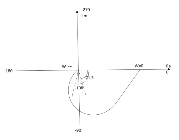
Fig 2 Polar Plot for T(S) = 1/(S+1)(S+2)
Intersection of polar plot with imaginary axis will be when real part of Transfer function = 0
M = 1/(jw + 1)(jw + 2)
= 1/-w2 + j3w + 2
Real part
Re(M) = 1/(2-w2)+j3w x (2-w2)-3jw/(2-w2)-3jw
Re(M) = (2-w2)/(2-w2+9w2) - 3jw/(2-w2) +9w2
Equating Real part = 0
(2-w2)/(2-w2)+ 9w2 = 0
W = +-√2
For w=√2 real part on the polar plot becomes zero.
So, polar plot intersects imaginary axis at w=√2 at φ = -900
Q3) Plot polar plot for T(S) = 1/(S+1)(S+2)(S+3)
A3)
(1). Substitute S =jw
(2). M = 1/√1+w2 √4+w2 √9+w2
(3). Φ = -tan-1w – tan-1 w/2 – tan-1w/3
WMφ
00.160
10.1-900
20.04-142.10
∞0-270
(4). Intersection of Polar plot with Real axis
M = 1/(S+1)(S+2)(S+3)
= 1/S3+6S2+11S+6
=1/(jw)2+6(jw)2+11jw+6
= 1/(6-6w2)+j(11w-w3)
Re(M) = 0 [Intersection with imaginary axis ]
M = 6-6w2/(6-6w2)2+(11w-w2)2 - j(11w-w3)/(6-6w2)2+(11w-w2)2
Re(M) = 0
6-6w2 = 0
w=1
Im(M) = 0[Intersection with Real axis]
11w = w3
The plot is shown in fig 3

Fig 3 Polar Plot for T(S) = 1/(S+1)(S+2)(S+3)
Q4) For T(S) = 1/S(S+1) plot polar plot?
A4)
(1). M = 1/W√1+w2
(2). Φ = -900 –
Tan -1(W/T)
WMφ
0∞-900
10.707-1350
20.45-153.40
∞0-1800
The plot is shown in fig.4

Fig 4 Polar Plot for T(S) = 1/S(S+1)
Q5) For T(s) = 1/S2(S+1) plot polar plot?
A5)
(1). M = 1/w2√1+jw
(2). Φ = -1800 – tan-1W/T
The plot is shown in fig. 5

Fig 5 Polar Plot for T(s) = 1/S2(S+1)
Q6) Sketch the bode plot for transfer function
G(S) = 
A6)
Replace S = j
G(j =
= 
This is type 0 system. So initial slope is 0 dB decade. The starting point is given as
20 log10 K = 20 log10 1000
= 60 dB
Corner frequency  1 =
1 =  = 10 rad/sec
 2 =
2 =  = 1000 rad/sec
Slope after  1 will be -20 dB/decade till second corner frequency i.e
  2 after
  2 the slope will be -40 dB/decade (-20+(-20)) as there are poles
For phase plot
 = tan-1 0.1
 - tan-1 0.001
For phase plot


100-900
200-9.450
300-104.80
400-110.360
500-115.420
600-120.00
700-124.170
800-127.940
900-131.350
1000 -134.420
The plot is shown in figure 6.
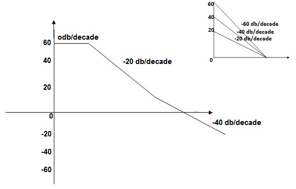
Fig 6. Magnitude Plot for G(S) = 
Q7) For the given transfer function determine
G(S) = 
Gain cross over frequency phase cross over frequency phase mergence and gain margin
A7)
Initial slope = 1
N = 1, (K)1/N = 2
K = 2
Corner frequency
 1 =
1 =  = 2 (slope -20 dB/decade
 2 =
2 =  = 20 (slope -40 dB/decade

Phase
 = tan-1
 - tan-1 0.5
  - tan-1 0.05
 = 900- tan-1 0.5
  - tan-1 0.05


1-119.430
5-172.230
10-195.250
15-209.270
20-219.30
25-226.760
30-232.490
35-236.980
40-240.570
45-243.490
50-245.910
Finding  gc (gain cross over frequency
M = 
4 =  2 (
2 ( (
(
 6 (6.25
 104) + 0.252
 4 +
4 + 2 = 4
2 = 4
Let  2 = x
2 = x
X3 (6.25 104) + 0.252
 2 + x = 4
X1 = 2.46
X2 = -399.9
X3 = -6.50
For x1 = 2.46
 gc = 3.99 rad/sec(from plot )
For phase margin
PM = 1800 - 
 = 900 – tan-1 (0.5×
 gc) – tan-1 (0.05 ×
  gc)
gc)
= -164.50
PM = 1800 - 164.50
= 15.50
For phase cross over frequency ( pc)
pc)
 = 900 – tan-1 (0.5
  ) – tan-1 (0.05
  )
)
-1800 = -900 – tan-1 (0.5  pc) – tan-1 (0.05
  pc)
pc)
-900 – tan-1 (0.5  pc) – tan-1 (0.05
  pc)
pc)
Taking than on both sides
Tan 900 = tan-1
Let tan-1 0.5  pc = A, tan-1 0.05
  pc = B
 = 00
= 00
 = 0
= 0
1 =0.5  pc 0.05
 pc
pc
 pc = 6.32 rad/sec
The plot is shown in figure 7.

Fig 7. Magnitude Plot for G(S) = 
Q8) For the given transfer function
G(S) = 
Plot the rode plot find PM and GM
A8)
T1 = 0.5  1 =
1 =  = 2 rad/sec
Zero so, slope (20 dB/decade)
T2 = 0.2  2 =
2 =  = 5 rad/sec
Pole, so slope (-20 dB/decade)
T3 = 0.1 = T4 = 0.1
 3 =
3 =  4 = 10 (2 pole ) (-40 db/decade)
1. Initial slope 0 dB/decade till  1 = 2 rad/sec
2. From  1 to
1 to 2 (i.e. 2 rad /sec to 5 rad/sec) slope will be 20 dB/decade
3. From  2 to
2 to  3 the slope will be 0 dB/decade (20 + (-20))
4. From  3 ,
3 , 4 the slope will be -40 dB/decade (0-20-20)
Phase plot
 = tan-1 0.5
 - tan-1 0.2
 - tan-1 0.1
 - tan-1 0.1


500-177.30
1000-178.60
1500-179.10
2000-179.40
2500-179.50
3000-179.530
3500-179.60
GM = 00
PM = 61.460
The plot is shown in figure 8.


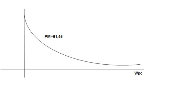
Fig 8. Magnitude and Phase plot for G(S) = 
Q8) For the given transfer function plot the bode plot (magnitude plot)
G(S) = 
A9)
Given transfer function
G(S) = 
Converting above transfer function to standard from
G(S) = 
= 
1. As type 1 system, so initial slope will be -20 dB/decade
2. Final slope will be -60 dB/decade as order of system decides the final slope
3. Corner frequency
T1 =  ,
,  11= 5 (zero)
T2 = 1,  2 = 1 (pole)
4. Initial slope will cut zero dB axis at
(K)1/N = 10
i.e  = 10
= 10
5. Finding  n and
n and 
T(S) = 
T(S)= 
Comparing with standard second order system equation
S2+2 ns +
ns + n2
n2
 n = 11 rad/sec
 n = 5
n = 5
 11 = 5
 =
=  = 0.27
6. Maximum error
M = -20 log 2
= +6.5 dB
7. As K = 10, so whole plot will shift by 20 log 10 10 = 20 Db
The plot is shown in figure 9.

Fig 9. Magnitude plot for G(S) = 
Q10) For the given plot determine the transfer function
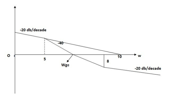
Fig 10 Magnitude plot for Q9
A10)
From figure 10, we can conclude that
1. Initial slope = -20 dB/decade so type -1
2. Initial slope alls 0 dB axis at  = 10 so
K1/N N = 1
(K)1/N = 10.
3. Corner frequency
 1 =
1 =  = 0.2 rad/sec
 2 =
2 =  = 0.125 rad/sec
4. At  = 5 the slope becomes -40 dB/decade, so there is a pole at
  = 5 as slope changes from -20 dB/decade to -40 dB/decade
5. At  = 8 the slope changes from -40 dB/decade to -20 dB/decade hence is a zero at
  = 8 (-40+(+20)=20)
6. Hence transfer function is
T(S) = 
Q9) For the transfer function below plot the Nyquist plot and also comment on stability? G(S) = 1/S+1
A11)
N = Z – P (No pole of right half of S plane P = 0)
P = 0, N = Z
NYQUIST PATH:
P1 = W – (0 to - ∞)
P2 = ϴ( - π/2 to 0 to π/2 )
P3 = W(+∞ to 0)
Substituting S = jw
G(jw) = 1/jw + 1
M = 1/√1+W2
Φ = -tan-1(W/I)
For P1: W(0 to -∞)
WMφ
010
-11/√2+450
-∞0+900
Path P2:
W = Rejϴ R ∞ϴ -π/2 to 0 to π/2
G(jw) = 1/1+jw
= 1/1+j(Rejϴ) (neglecting 1 as R ∞)
M = 1/Rejϴ = 1/R e-jϴ
M = 0 e-jϴ = 0
Path P3:
W = -∞ to 0
M = 1/√1+W2, φ = -tan-1(W/I)
WMφ
∞0-900
11/√2-450
0100
The Nyquist Plot is shown in fig 11.
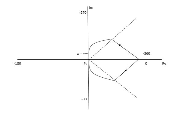
Fig 11. Nyquist plot for G(S) = 1/S+1
From plot we can see that -1 is not encircled so, N = 0
But N = Z, Z = 0
So, system is stable.
Q10) For the transfer function below plot the Nyquist Plot and comment on stability G(S) = 1/(S + 4)(S + 5)
A12)
N = Z – P, P = 0, No pole on right half of S-plane
N = Z
NYQUIST PATH
P1 = W(0 to -∞)
P2 = ϴ(-π/2 to 0 to +π/2)
P3 = W(∞ to 0)
Path P1 W(0 to -∞)
M = 1/√42 + w2 √52 + w2
Φ = -tan-1(W/4) – tan-1(W/5)
WMΦ
01/2000
-10.04725.350
-∞0+1800
Path P3 will be the mirror image across the real axis.
Path P2: ϴ(-π/2 to 0 to +π/2)
S = Rejϴ
G(S) = 1/(Rejϴ + 4)( Rejϴ + 5)
R∞
= 1/ R2e2jϴ = 0.e-j2ϴ = 0
The plot is shown in fig 12. From plot N=0, Z=0, system stable.
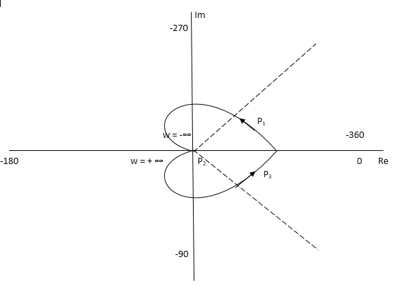
Fig 12. Nyquist plot for G(S) = 1/(S + 4)(S + 5)
Q11) For the given transfer function, plot the Nyquist plot and comment on stability G(S) = k/S2(S + 10)?
A13)
As the poles exists at origin. So, first time we do not include poles in Nyquist plot. Then check the stability for second case we include the poles at origin in Nyquist path. Then again check the stability.
PART – 1: Not including poles at origin in the Nyquist Path.

P1 W(∞ Ɛ) where Ɛ 0
P2 S = Ɛejϴϴ(+π/2 to 0 to -π/2)
P3 W = -Ɛ to -∞
P4 S = Rejϴ, R ∞, ϴ = -π/2 to 0 to +π/2
For P1
M = 1/w.w√102 + w2 = 1/w2√102 + w2
Φ = -1800 – tan-1(w/10)
WMΦ
∞0-3 π/2
Ɛ∞-1800
Path P3 will be mirror image of P1 about Real axis.
G(Ɛ ejϴ) = 1/( Ɛ ejϴ)2(Ɛ ejϴ + 10)
Ɛ 0, ϴ = π/2 to 0 to -π/2
= 1/ Ɛ2 e2jϴ(Ɛ ejϴ + 10)
= ∞.e-j2ϴ [ -2ϴ = -π to 0 to +π ]
Path P2 will be formed by rotating through -π to 0 to +π
Path P4 S = Rejϴ R ∞ ϴ = -π/2 to 0 to +π/2
G(Rejϴ) = 1/ (Rejϴ)2(10 + Rejϴ)
= 0
N = Z – P
No poles on right half of S plane so, P = 0
N = Z – 0

Fig 13. Nyquist plot for G(S) = k/S2(S + 10)
But from plot shown in fig 13. It is clear that number of encirclements in Anticlockwise direction. So,
N = 2
N = Z – P
2 = Z – 0
Z = 2
Hence, system unstable.
PART 2 Including poles at origin in the Nyquist Path.

P1 W(∞ to Ɛ) Ɛ 0
P2 S = ƐejϴƐ 0 ϴ(+π/2 to +π to +3π/2)
P3 W(-Ɛ to -∞) Ɛ 0
P4 S = Rejϴ, R ∞, ϴ(3π/2 to 2π to +5π/2)
M = 1/W2√102 + W2 , φ = - π – tan-1(W/10)
P1W(∞ to Ɛ)
WMφ
∞0-3 π/2
Ɛ∞-1800
P3( mirror image of P1)
P2S = Ɛejϴ
G(Ɛejϴ) = 1/ Ɛ2e2jϴ(10 + Ɛejϴ)
Ɛ 0
G(Ɛejϴ) = 1/ Ɛ2e2jϴ(10)
= ∞. e-j2ϴϴ(π/2 to π to 3π/2)
-2ϴ = (-π to -2π to -3π)
P4 = 0
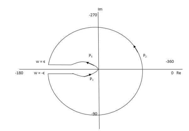
Fig 14. Nyquist Plot for G(S) = k/S2(S + 10)
The plot is shown in fig. From the plot it is clear that there is no encirclement of -1 in Nyquist path. (N = 0). But the two poles at origin lies to the right half of S-plane in Nyquist path.(P = 2)[see path P2]
N = Z – P
0 = Z – 2
Z = 2
Hence, system is unstable.
Path P2 will be formed by rotating through -π to -2π to -3π
Q12) Explain relation between time and frequency response?
A14) The calculation of system parameters for higher order systems is difficult in time domain analysis. This can be overcome by frequency domain analysis. As the frequency response of a linear time invariant system is independent of amplitude and phase of the input test signal. The effect of noise and parameter variation in frequency domain can be easily computed.
In frequency response can be determine by calculating the phase and amplitude oof the given system transfer function. If a sinusoidal signal XG(j )sin
)sin t then its amplitude will be
C(t) = XG(j )sin
)sin t
t
= X|G(j )|
)| sin
sin t
t
Magnitude = |G(j )|
)|
Phase = 
In polar form = |G(j )|
)|
The transfer function of second order system is shown as
C(S)/R(S) = W2n / S2 + 2ξWnS + W2n - - (1)
ξ = Ramping factor
Wn = Undamped natural frequency for frequency response let S = jw
C(jw) / R(jw) = W2n / (jw)2 + 2 ξWn(jw) + W2n
Let U = W/Wn above equation becomes
T(jw) = W2n / 1 – U2 + j2 ξU
So,
| T(jw) | = M = 1/√(1 – u2)2 + (2ξU)2 - - (2)
T(jw) = φ = -tan-1[ 2ξu/(1-u2)] - - (3)
For sinusoidal input the output response for the system is given by
C(t) = 1/√(1-u2)2 + (2ξu)2Sin[wt - tan-1 2ξu/1-u2] - - (4)
The frequency where M has the peak value is known as Resonant frequency Wn. This frequency is given as (from eqn (2)).
DM/du|u=ur = Wr = Wn√(1-2ξ2) - - (5)
From equation(2) the maximum value of magnitude is known as Resonant peak.
Mr = 1/2ξ√1-ξ2 - - (6)
The phase angle at resonant frequency is given as
Φr = - tan-1 [√1-2ξ2/ ξ] - - (7)
As we already know for step response of second order system the value of damped frequency and peak overshoot are given as
Wd = Wn√1-ξ2 - - (8)
Mp = e- πξ2|√1-ξ2 - - (9)


Fig 15. Frequency Domain Specification
The comparison of Mr and Mp is shown in figure. The two performance indices are correlated as both are functions of the damping factor ξ only. When subjected to step input the system with given value of Mr of its frequency response will exhibit a corresponding value of Mp.
Similarly the correlation of Wr and Wd is shown in figure for the given input step response [ from eqn(5) & eqn(8) ]
Wr/Wd = √(1- 2ξ2)/(1-ξ2)
Mp = Peak overshoot of step response
Mr = Resonant Peak of frequency response
Wr = Resonant frequency of Frequency response
Wd = Damping frequency of oscillation of step response.
From fig(17) it is clear that for ξ> 1/2, value of Mr does not exists.
Q13) For the following system shown below find the phase margin and gain margin if the value of k=500 by using Nyquist plot.

A15)
G(s)H(s) = 500/s(s+6)(s+9)
The polar plot for above OLTF is shown in figure below.

Fig 16. Polar Plot for given system
From figure we see A=0.6,
The GM in dB = -20logA.
= 4.43dB
PM = 1800-1650
= 150
Q14) For the system shown in figure, find the GM and PM using Nyquist plot for k=10. Find also range of k for stability?

A16)
The transfer function is G(s) H(s) = 10(s+2(s+4)/s(s2 – 3s+10)
As the OLTF is unstable system so PM and GM concepts cannot be applied.
G(jω) H(jω) = 10(jω+2) (jω+4)/ jω(-ω2 -3 jω+10)
| G(jω) H(jω)|= 10(√4+ω2)( √16+ω2)/ ω√[(10-ω)2+9 ω2]
 G(jω)H(jω) = -900 +tan-1(ω/2) + tan-1(ω/4) - tan-1 (-3ω/10- ω2)
The polar plot for above system is shown below.
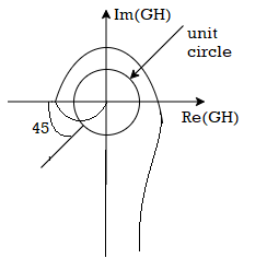
Fig 17. Polar plot for the given system
From figure we have A=2.6 and ɸ =-1350
The GM in dB = -20logA.
= -8.3dB
As GM is negative it indicates that system is open loop unstable.
PM = 1800-1650 = 450
Q15) Write short note on Nicholas chart?
A17)
The Nichols plot is named after the American engineer N.B Nichols who formulated this plot. Compensators can be designed using Nichols plot. Nichols plot technique is however also used in designing of dc motor. This is used in signal processing and control design. Nyquist plot in complex plane shows how phase of transfer function and frequency variation of magnitude are related. • Angle of positive real axis determines the phase and distance from origin of complex plane determines the gain.
Advantages
- Gain and phase margin can be determined easily and also graphically.
- Closed loop frequency response is obtained from open loop frequency response.
- Gain of the system can be adjusted to suitable values.
- Nichols chart provides frequency domain specifications.
Disadvantage
Using Nichols plot small changes in gain cannot be encountered easily.
Q16) What are M circles? Derive its equation for forming circle?
A18)
Constant magnitude loci that are M-circles and constant phase angle loci that are N-circles are the fundamental components. The constant M and constant N circles in G (jω) plane can be used for the analysis and design of control systems. However, the constant M and constant N circles in gain phase plane are prepared for system design and analysis as these plots supply information with fewer manipulations. Gain phase plane is the graph having gain in decibel along the ordinate (vertical axis) and phase angle along the abscissa (horizontal axis).
For Constant M Circle
For a system with unity feedback having transfer function
T(s)= G(s)/1+G(s)
Replace s=jω
T(jω) = G(jω)/1+G(jω)
But we can write G(jω)= X(jω)+jY(jω)
The closed loop transfer function T(s) is
T(jω) = X+jY/1+X+jY= Mejα
M= |X+jY|/|1+X+jY|
M2=X2+Y2/(1+X2) + Y2
Solving above equation we get
[X-(M2/1-M2)]2 + Y2 = ([M/1-M2)]2
This is equation of circle with centre (M2/1-M2),0 and radius M/1-M2
When M<1, M decreases the radius of the circle decreases and centres located on positive real axis shifts towards origin. When M=0 the radius becomes 0 and the centre (0,0). This is shown in figure above.

Fig 18. Constant M circle
Q17) For T(S) = 1/S plot polar plot?
A19)
(1). S = jw
(2). M = 1/W
(3). Φ = -tan-1(W/O) = -900
WMφ
0∞-900
11-900
20.5-900
∞0-900
The plot is shown in fig. 19.

Fig 19. Polar plot for T(S) = 1/S
Q18) Define the relationship between time and frequency response?
A20)
The calculation of system parameters for higher order systems is difficult in time domain analysis. This can be overcome by frequency domain analysis. As the frequency response of a linear time invariant system is independent of amplitude and phase of the input test signal. The effect of noise and parameter variation in frequency domain can be easily computed.
In frequency response can be determine by calculating the phase and amplitude oof the given system transfer function. If a sinusoidal signal XG(j )sin
)sin t then its amplitude will be
C(t) = XG(j )sin
)sin t
t
= X|G(j )|
)| sin
sin t
t
Magnitude = |G(j )|
)|
Phase = 
In polar form = |G(j )|
)|
The transfer function of second order system is shown as
C(S)/R(S) = W2n / S2 + 2ξWnS + W2n - - (1)
ξ = Ramping factor
Wn = Undamped natural frequency for frequency response let S = jw
C(jw) / R(jw) = W2n / (jw)2 + 2 ξWn(jw) + W2n
Let U = W/Wn above equation becomes
T(jw) = W2n / 1 – U2 + j2 ξU
So,
| T(jw) | = M = 1/√(1 – u2)2 + (2ξU)2 - - (2)
T(jw) = φ = -tan-1[ 2ξu/(1-u2)] - - (3)
For sinusoidal input the output response for the system is given by
C(t) = 1/√(1-u2)2 + (2ξu)2Sin[wt - tan-1 2ξu/1-u2] - - (4)
The frequency where M has the peak value is known as Resonant frequency Wn. This frequency is given as (from eqn (2)).
DM/du|u=ur = Wr = Wn√(1-2ξ2) - - (5)
From equation(2) the maximum value of magnitude is known as Resonant peak.
Mr = 1/2ξ√1-ξ2 - - (6)
The phase angle at resonant frequency is given as
Φr = - tan-1 [√1-2ξ2/ ξ] - - (7)
As we already know for step response of second order system the value of damped frequency and peak overshoot are given as
Wd = Wn√1-ξ2 - - (8)
Mp = e- πξ2|√1-ξ2 - - (9)

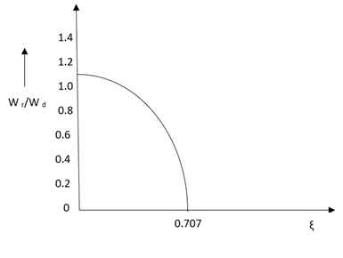
Fig 20. Frequency Domain Specification
The comparison of Mr and Mp is shown in figure. The two performance indices are correlated as both are functions of the damping factor ξ only. When subjected to step input the system with given value of Mr of its frequency response will exhibit a corresponding value of Mp.
Similarly the correlation of Wr and Wd is shown in figure for the given input step response [ from eqn(5) & eqn(8) ]
Wr/Wd = √(1- 2ξ2)/(1-ξ2)
Mp = Peak overshoot of step response
Mr = Resonant Peak of frequency response
Wr = Resonant frequency of Frequency response
Wd = Damping frequency of oscillation of step response.
From fig(1) it is clear that for ξ> 1/2, value of Mr does not exists.