UNIT-5
CURVES AND FRACTALS
Question-1: Explain analysis of curves in computer graphics with blending function.
Sol:
A curve is an infinite large set of points.
Each point has two neighbors except endpoints.
The classification of the curve is as follows:
Explicit curve
Implicit curve
Parametric curve
Blending function:
The function that is combined with control point to sense the influence each control point has over each curve point.
The influences are blended to yield the final curve point and this function is called as blending function.
The blending function is used to generate the bezier curve.
The curve points are weighted average of the control point.
The blending function gives the weight.
The evaluation of the four-blending function at particular parameter value t to get four number that are weights in weighted sum of the four control points.
Question-2: Explain the blending function of curves in graphics.
Sol:
The function that is combined with control point to sense the influence each control point has over each curve point.
The influences are blended to yield the final curve point and this function is called as blending function.
The blending function is used to generate the bezier curve.
The curve points are weighted average of the control point.
The blending function gives the weight.
The evaluation of the four-blending function at particular parameter value t to get four number that are weights in weighted sum of the four control points.
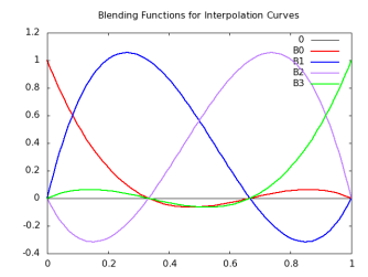
Following equation gives the curve P(t) as weighted sum of the four control point.
P(t)=B0(t) * P0 + B1(t) * P1 + B2(t) * P2 + B3(t) * P3
Following are blending functions for interpolating curves:
B0(t)= -9/2 (t-1/3)(t-2/3)(t-1)
B1(t)=27/2 t(t – 2/3) (t - 1)
B2(t)= -27/2 t (t – 2/3) (t - 1)
B3(t)= -9/2 t (t – 1/3) (t – 2/3)
Following is the function for interpolation curves:
Question-3: Explain interpolation and approximation.
Sol:
The interpolation is filling in frames between the key frames.
It uses the polynomial interpolation to draw images semi automatically.
It is a generating principle which enables to model connected curve segments from the discrete ordered sets of points in the extended space.
Question-4: What is B-spline curves? Explain with properties.
Sol:
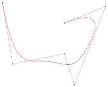
B-spline curve overcomes the limitation of Bezier curve as Bezier curve has limited flexibility.
It is a special case of Berstein basis.
It is non-global method.
It consists of linear
combination of control points Pi and B-spline basis function Ni.
The mathematical representation of B-spline curve is,
C(t) = ∑ Pi * N(i,k)(t)
Where summation limitation is n to i=0 and n >= k-1, t belongs to (tk - 1, tn + 1)
Here k is order of polynomial segments of B-spline curve.
N(i,k)(t) it is an normalized B-spline blending function.
Properties of B-spline curve:
Question-5: What is Bezeir curve in computer graphics?
Sol:
The Bezier curve are developed by French engineer Pierre Bezier.
The Bezier curve is generated under the control of other points.
To generate the Bezier curve approximate tangents are used by using control points.
The mathematical representation of Bezier curve is,
∑ Pi * B ni (t) where summation from n to k=0
Pi is the set of points and B(t) is berstein polynomials as B(t)= (n , i)(1 - t)n-I * ti
The simple beizer curve is a straight line from P0 to P1.
A quadratic Bezier curve has three control points.
A cubic Bezier curve is determined by four control points.

Properties of Bezier curve:
Question-6: Short note on fractal.
Sol:
The fragmented geometric shape that can be split into parts.
Fractal is the complex picture that is generated by computer from one formula.
Fractals are created using iteration.
The formula of fractal repeats again and again with slightly different values.
Question-7: Explain the classification of fractals.
Sol:
The fractals can be classified as:
Self-Similar Fractal:
These fractals are scaled down the version of entire object.
The overall fractals are scaled by the applying the scaling parameter s to the initial shape.
It is all over the user to choose the same scaling factor s for all subparts or different scaling factors for different scaled down parts.
In sub class of self-similar fractal the user can use the random variation to the scaled down sub parts.
This fractalare used to model tree, shrubs and other plants.
Self-Affine Fractal:
The self-affine fractals are scaled down with different scaling parameters as Sx, Sy and Sz in different coordinate direction.
We can apply random variations to obtain self-affine fractals.
This fractals are used to model water, clouds and terrain.
Invariant:
The invariant fractals uses the non-linear transformation.
It includes self-squaring function such as Mandelbrot set.
It uses inversion procedure to form squaring function and self-inverse fractals.
Question-8: Short note on fractal generation in graphics.
Sol:
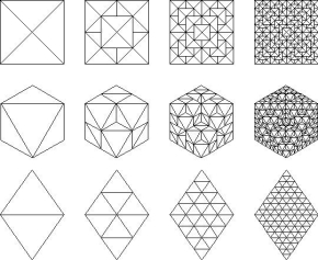
The fractal generation can be done by repeating same shape again and again.
Following figure shows the fractal generation by repeating the shape.

Question-9: Explain snowflake fractal.
Sol:
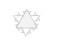
It is known as Koch curve, Koch star or Koch island.
It is mathematical curve and described earliest than the other fractals.
Following are some step to create snowflake fractal.
Step 1: draw a triangle.
Step 2: divide each side in three equal parts.
Step 3: draw an equilateral triangle on each middle part.
Step 4: divide each outer side into three and second generation of triangles covers the bit of first.
Step 5: repeat the process to get the snowflake fractal.
Following figure shows the snowflake fractal.
Question-10: Write short note on triadic curve fractal.
Sol:
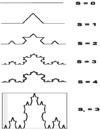
The triadic Koch curve is constructed as the limit of sequence of simple iterative steps.
Starting with line unit length.
At each stage, middle third of the line length ƛ is replaced by equal segments of length ƛ/3 to form sides of an equilateral triangle.
Proceeding for an infinite number of steps one obtains triadic Koch curve.
Following figure shows the triadic curve.
Question-11: Explain the Hilbert curve in graphics.
Sol:
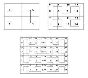
It is also known as Hilbert space filling curve.
It is continuous fractal space filling curve.
It is developed by German mathematician David Hilbert.
As it is a space filling algorithm its Hausdroff dimension is 2.
It has unit square image which has dimension as 2.
Its graph is compact set homeomorphic to the closest interval.
Following figure shows the Hilbert curve.
Question-12: Write applications of the fractal.
Sol:
Following are the applications of the fractal.