undefined | unit 3 searching and sorting

FDS

UNIT 3

QUESTIONS

Q1 Explain sequential and binary search

1. Linear /Sequential search

Linear search is the simplest searching algorithm that searches for an element in a list in sequential order. We start at one end and check every element until the desired element is not found.

Algorithm

Linear Search (Array A, Value x)

Step 1: Set i to 1

Step 2: if i> n then go to step 7

Step 3: if A[i] = x, then go to step 6

Step 4: Set i to i + 1

Step 5: Go to Step 2

Step 6: Print Element x Found at index i and go to step 8

Step 7: Print element not found

Step 8: Exit

Array to be search for

Start from element k with element x

K=1

K≠2

K≠4

K≠0

2. If x==k then return index

K=1

3. Else return ; element not found

Time complexity of linear search O(n)

Space complexity of linear search O(1)

Where n is no. of elements

2. Binary search

Binary Search is a searching algorithm for finding an element's position in a sorted array.

A binary search algorithm is a technique for finding particular value in alinar array, by ruling out half of the data at each step.

A binary search finds the median, makes comparisons’ to determine whether the desired value comes before or after it, then searches the remaining half in the same manner.

Algorithm

Function Binarysearch(a,value,left ,right)

If right<left

Return not found

Mid= floor((right-left)/2)+ left;

If a[mid]=value

Return mid

If value<a[mid]

Return binarysearch(a,value,left,mid-1)

Else

Return binarysearch(a,value,mid+1,right)

1. The array in which searching is to be performed is

Element to find x=4

2. Set two pointers low and high at the lowest and the highest positions respectively

Low high

3. Find the middle element mid=arr (low+high)/2= 6

Mid

4.If x == mid, then return mid. Else, compare the element to be searched with m.

5. If x > mid, compare x with the middle element of the elements on the right side of mid. This is done by setting low to low = mid + 1.

6. Else, compare x with the middle element of the elements on the left side of mid. This is done by setting high to high = mid - 1.

Low high

7. Repeat steps 3 to 6 until low meets high.

Low mid high

8 if x==mid return

X=mid

Binary search complexities

Time Complexities

Best case complexity: O(1)

Average case complexity: O(log n)

Worst case complexity: O(log n)

Space Complexity

The space complexity of the binary search is O(n).

Q2 Explain bubble sort

1. Bubble sort

Bubble sort is an algorithm that compares the adjacent elements and swaps their positions if they are not in the intended order. The order can be ascending or descending

Algorithm

bubbleSort(array)

for i<- 1 to indexOfLastUnsortedElement-1
if leftElement>rightElement
swap leftElement and rightElement

end bubbleSort

Starting from the first index, compare the first and the second elements.If the first element is greater than the second element, they are swapped.

Now, compare the second and the third elements. Swap them if they are not in order.

The above process goes on until the last element.

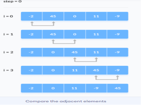
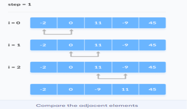
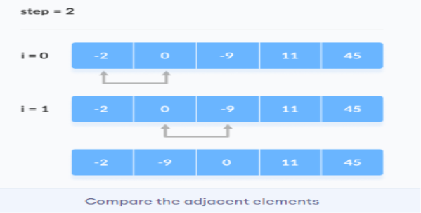
$C:\Users\Kilua Zoldyck\Pictures\b1.png$

2. The same process goes on for the remaining iterations. After each iteration, the largest element among the unsorted elements is placed at the end.

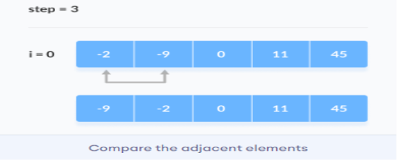
In each iteration, the comparison takes place up to the last unsorted element.

The array is sorted when all the unsorted elements are placed at their correct positions.

$C:\Users\Kilua Zoldyck\Pictures\b2.png$

$C:\Users\Kilua Zoldyck\Pictures\b3.png$

$C:\Users\Kilua Zoldyck\Pictures\b4.png$

Time Complexities:

Worst Case Complexity: O(n2)

.Best Case Complexity: O(n)
Average Case Complexity: O(n2)

Space Complexity:

Space complexity is O(1) because an extra variable temp is used for swapping.

Bubble Sort Applications

Bubble sort is used in the following cases where

The complexity of the code does not matter.

A short code is preferred.

Q3 Explain insertion sort with example

Insertion sort

Insertion sort is a comparison sort in which the sorted array is built one entry at a time.

It is less efficient on large lists than more advanced algorithms such as quick sort ,heap sort or merge sort

This algorithm does not require extra memory

For insertion sort the worst case running time is O(n^2) and best case running time is O(n).

Insertion sort use no extra memory it sort in place.

The time of insertion sort is depends on the original order of input.

Algorithm

insertionSort(array)

mark first element as sorted

for each unsorted element X

'extract' the element X

for j <- lastSortedIndex down to 0

if current element j > X

move sorted element to the right by 1

break loop and insert X here

end insertionSort

1. The first element in the array is assumed to be sorted. Take the second element and store it separately in key.

Array

$C:\Users\Kilua Zoldyck\Pictures\a1.png$

Compare key with the first element. If the first element is greater than key, then key is placed in front of the first element.

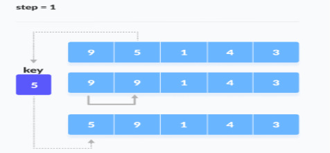
$C:\Users\Kilua Zoldyck\Pictures\a2.png$

If the first element is greater than key, then key is placed in front of the first element

2. Now, the first two elements are sorted. Take the third element and compare it with the elements on the left of it. Placed it just behind the element smaller than it. If there is no element smaller than it, then place it at the beginning of the array.

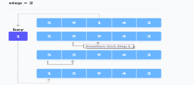
$C:\Users\Kilua Zoldyck\Pictures\a3.png$

Place 1 at the beginning

3. Similarly, place every unsorted element at its correct position.

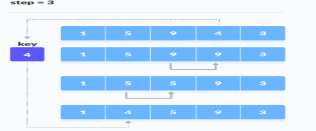
$C:\Users\Kilua Zoldyck\Pictures\a5.png$

Place 4 behind 1

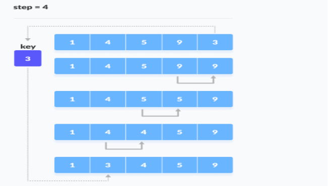
$C:\Users\Kilua Zoldyck\Pictures\a6.png$

Place 3 behind 1 and the array is sorted

Q4 Explain quick sort with example

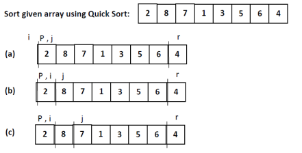
Quick sort

Algorithm

quickSort(array, leftmostIndex, rightmostIndex)

if (leftmostIndex<rightmostIndex)
pivotIndex<- partition(array,leftmostIndex, rightmostIndex)
quickSort(array, leftmostIndex, pivotIndex)
quickSort(array, pivotIndex + 1, rightmostIndex)

partition(array, leftmostIndex, rightmostIndex)

set rightmostIndex as pivotIndex
storeIndex<- leftmostIndex – 1
for i<- leftmostIndex + 1 to rightmostIndex
if element[i] <pivotElement
swap element[i] and element[storeIndex]
storeIndex++
swap pivotElement and element[storeIndex+1]
return storeIndex + 1

Quick sort

Quicksort is that the currently fastest known algorithm and is usually the simplest practical choice for sorting, as its average expected time period is O(n log(n)).

Pick a component, called a pivot, from the array.

Reorder the array in order that all elements with values but the pivot precede the pivot, while all elements with values greater than the pivot come after it (equal values can go either way). After this partitioning, the pivot is in its final position. This is often called the partition operation.

Recursively apply the above steps to the sub-array of elements with smaller values and separately to the sub-array of elements with greater values.

Quicksort, like merge sort, may be a divide-and-conquer recursive algorithm.

The basic divide-and-conquer process for sorting a sub array A[i..j] is summarized within the following three easy steps:

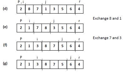
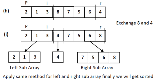
Divide: Partition T[i..j] Into two sub arrays T[i..l-1] and T[l+1… j] such each element of T[i..l-1] is less than or adequate to T[l], which is, in turn, but or adequate to each element of T[l+1… j]. Compute the index l as a part of this partitioning procedure
Conquer: Sort the 2 sub arrays T[i..l-1] and T[l+1… j] by recursive calls to quicksort.
Combine: Since the sub arrays are sorted in situ, no work is required to combing them: the whole arrayT[i..j], is now sorted.

$C:\Users\Kilua Zoldyck\Pictures\q1.png$

$C:\Users\Kilua Zoldyck\Pictures\q2.png$

$C:\Users\Kilua Zoldyck\Pictures\q3.png$

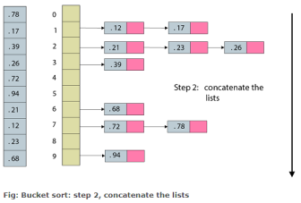
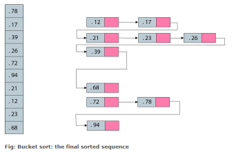
Q5 Explain bucket sort algorithm with example

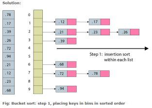
Bucket Sort

Algorithm

bucketSort()

create N buckets each of which can hold a range of values
for all the buckets
initialize each bucket with 0 values
for all the buckets
put elements into buckets matching the range
for all the buckets
sort elements in each bucket
gather elements from each bucket

end bucketSort

bucket sort

array A = (0.78, 0.17, 0.39, 0.26, 0.72, 0.94, 0.21, 0.12, 0.23, 068)

$C:\Users\Kilua Zoldyck\Pictures\bn1.png$ $C:\Users\Kilua Zoldyck\Pictures\b2.png$

$C:\Users\Kilua Zoldyck\Pictures\b3.png$

Q6. Explain radix sort?

Radix Sort

Algorithm

radixSort(array)

d <- maximum number of digits in the largest element
create d buckets of size 0-9
for i<- 0 to d
sort the elements according to ith place digits using countingSort

countingSort(array, d)

max <- find largest element among dth place elements
initialize count array with all zero
for j <- 0 to size
find the total count of each unique digit in dth place of elements and
store the count at jth index in count array
for i<- 1 to max
find the cumulative sum and store it in count array itself
for j <- size down to 1
restore the elements to array
decrease count of each element restored by 1

input array=[576, 494, 194,296,278,176, 954}

input

576 49[4] 9[5]4 [1]76 176

494 19[4] 5[7]6 [1]94 194

194 95[4] 1[7]6 [2]78 278

296 → 57[6] → 2[7]8 → [2]96→ 296

278 29[6] 4[9]4 [4]94 494

176 17[6] 1[9]4 [5]76 576

954 27[8] 2[9]6 [9]54 954

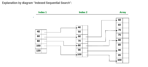
Q7 Explain indexed sequential search

Indexed sequential search

In this searching method, first of all, an index file is made, that contains some specific group or division of required record when the index is obtained, then the partial indexing takes less time because it's located during a specified group.

When the user makes an invitation for specific records it'll find that index group first where that specific record is recorded.

Characteristics of Indexed Sequential Search:

In Indexed Sequential Search a sorted index is about aside additionally to the array.

Each element within the index points to a block of elements within the array or another expanded index.

The index is searched 1st then the array and guides the search within the array.

Indexed Sequential Search actually does the indexing multiple time, like creating the index of an index.

$C:\Users\Kilua Zoldyck\Pictures\ss.png$

Time complexity of indexed sequential search

best case complexity is O(1)

worst case complexity is O(n)

Space complexity O(1)

Q8 What is counting sort?

Counting Sort

Counting sort assumes that each of the n inputs elements is an integer in the range 0 to k for some integer k. When k=O(n) time the sort runs in O(n) time.

The basic idea of counting sort is to determine for each input element x the number of elements less than x.

This information can be used to place elements x directly into its position in the output array

Algorithm

COUNTING-SORT(A,B,K)

For I← 0 to k

Do C[i]←0

For j←1 to length[A]

Do C[A[j]]← C[A[j]]+1

/* C[i] now contains the number of elements equal to i. */

For i← 1 to k

C[i] ← C[i] + C[i-1]

/* C[i] now contains the number of elements less than or equal to i. */

For j← length[A] down to 1

Do B[C[A[j]]] ←A[j]

C[A[j]] ←C[A[j]]-1

An important property of counting sort is that it is stable; numbers with the same value appear in the output array in the same order as they do in the input array

That is ties between two numbers are broken by the rule that whichever number appears first in the input array appears first in the output array.

Normally the property of stability is important only when satellite data are carried around with the element being sorted.

Find out the maximum element (let it be max) from the given array.

$C:\Users\Kilua Zoldyck\Pictures\cs1.png$

2. Initialize an array of length max+1 with all elements 0. This array is used for storing the count of the elements in the array.

$C:\Users\Kilua Zoldyck\Pictures\cs2.png$

3. Store the count of each element at their respective index in count array.

For example: if the count of element 3 is 2 then, 2 is stored in the 3rd position of count array. If element "5" is not present in the array, then 0 is stored in 5th position.

$C:\Users\Kilua Zoldyck\Pictures\cs3.png$

4. Store cumulative sum of the elements of the count array. It helps in placing the elements into the correct index of the sorted array.

$C:\Users\Kilua Zoldyck\Pictures\cs4.png$

5. Find the index of each element of the original array in the count array. This gives the cumulative count. Place the element at the index calculated as shown in figure below.

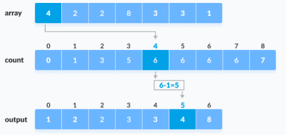
$C:\Users\Kilua Zoldyck\Pictures\cs5.png$

After placing each

Q9 Explain selection sort?

Selection sort

Selection sort is a sorting algorithm specifically an in place comparison sort.

It has O(n) complexity making it efficient on large lists

Implementation

Find the minimum value in the list

Swap it with the value in first position

Repeat the steps above for the rest of the list(starting at second and advance each time.

Algorithm

For i← 1 to n-1 do

Min j ←I;

Min x← A[i]

For j← i+1

If A[j] <min x then

Min j← j

Min x ←A[j]

A[i] ←min x

Set the first element as minimum. Select

Selection Sort Steps

First element as minimum

2. Compare minimum with the second element. If the second element is smaller than minimum, assign the second element as minimum.
Compare minimum with the third element. Again, if the third element is smaller, then assign minimum to the third element otherwise do nothing. The process goes on until the last element.

Selection Sort Steps Compare minimum with the remaining elements

3. After each iteration, minimum is placed in the front of the unsorted list. Selection Sort Steps

Swap the first with minimum

4. For each iteration, indexing starts from the first unsorted element. Step 1 to 3 are repeated until all the elements are placed at their correct positions.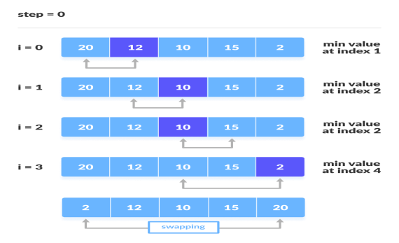 Selection Sort Steps

The first iteration

Selection sort steps

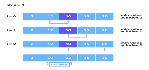
The second iteration

Selection sort steps

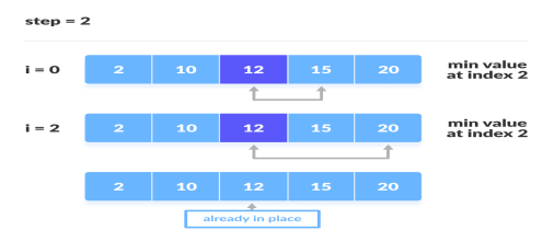
The third iteration

Selection sort steps

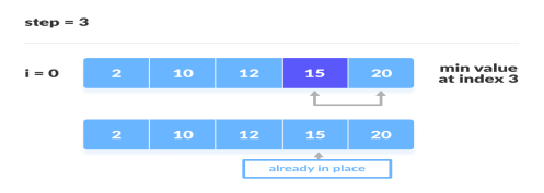
The fourth iteration

Q10 What is external and internal sorting?

There are two different categories in sorting:

Internal sorting

External sorting

Internal sorting:

If the input file is such it are often adjusted within the main memory directly, it's called internal sorting.

internal sorting stores the info to be sorted within the memory itself all the time when the sorting is ongoing

It is usually applied in cases where data can't be fit into the memory.

In internal sorting you'll randomly access elements from the memory while in external accessing data from the disks will take a while

Internal sorting are sort of sorting which is employed when the whole collection of knowledge is little enough that sorting can happen within main memory.

There’s no need for external memory for execution of sort program.

It is used when size of input is little

In internal sorting the info that has got to be sorted are going to be within the main memory always, implying faster access. Complete sorting will happen in main memory. Insertion sort, quick sort, heap sort, radix sort are often used for internal sorting

Examples:- Bubble sort, insertion sort,quicksort, heapsort

The sorting during which there's no got to use another storage structure because the data is manageable enough within the RAM.

External sorting:

If the input file is such it can't be adjusted within the memory entirely directly, it must be stored during a hard disc, diskette, or the other memory device. This is often called external sorting

.In external sorting it'll on disks, outside main memory. It are often because the info is large and can't be stored in main memory. While sorting the info will pulled over in chunks from disk to main memory.

Later all the sorted data are going to be merged and stored back to disk, where it can fit. External merge sort are often used here.

External sorting may be a term for a category of sorting algorithms which will handle massive amounts of knowledge.

External sorting is required when the info being sorted don't fit into the most memory of a computer (usually RAM) and instead, they need to reside within the slower external memory (usually a tough drive).

External sorting typically uses a hybrid sort-merge strategy. Within the sorting phase, chunks of knowledge sufficiently small to suit in main memory are read, sorted, and written bent a short lived file. Within the merge phase, the sorted sub-files are combined into one larger file.

But in external sorting data is loaded into the memory only it's required.

One example of external sorting is that the external merge sort algorithm, which sorts chunks that every slot in RAM, then merges the sorted chunks together.

We first divide the file into runs such the dimensions of a run is little enough to suit into main memory. Then sort each run in main memory using merge sort algorithm. Finally merge the resulting runs together into successively bigger runs, until the file is sorted.

Sign Up