UNIT-5

Graph and Symbol Table

Q1) What is graph explain in brief?

A1) A graph can be defined as group of vertices and edges that are used to connect these vertices. A graph can be seen as a cyclic tree, where the vertices (Nodes) maintain any complex relationship among them instead of having parent child relationship.

Definition

A graph G can be defined as an ordered set G(V, E) where V(G) represents the set of vertices and E(G) represents the set of edges which are used to connect these vertices.

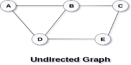
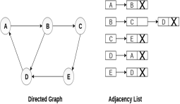
A Graph G(V, E) with 5 vertices (A, B, C, D, E) and six edges ((A,B), (B,C), (C,E), (E,D), (D,B), (D,A)) is shown in the following figure.

Directed and Undirected Graph

A graph can be directed or undirected. However, in an undirected graph, edges are not associated with the directions with them. An undirected graph is shown in the above figure since its edges are not attached with any of the directions. If an edge exists between vertex A and B then the vertices can be traversed from B to A as well as A to B.

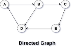
In a directed graph, edges form an ordered pair. Edges represent a specific path from some vertex A to another vertex B. Node A is called initial node while node B is called terminal node.

A directed graph is shown in the following figure.

Graph Terminology

Path

A path can be defined as the sequence of nodes that are followed in order to reach some terminal node V from the initial node U.

Closed Path

A path will be called as closed path if the initial node is same as terminal node. A path will be closed path if V0=VN.

Simple Path

If all the nodes of the graph are distinct with an exception V0=VN, then such path P is called as closed simple path.

Cycle

A cycle can be defined as the path which has no repeated edges or vertices except the first and last vertices.

Connected Graph

A connected graph is the one in which some path exists between every two vertices (u, v) in V. There are no isolated nodes in connected graph.

Complete Graph

A complete graph is the one in which every node is connected with all other nodes. A complete graph contain n(n-1)/2 edges where n is the number of nodes in the graph.

Weighted Graph

In a weighted graph, each edge is assigned with some data such as length or weight. The weight of an edge e can be given as w(e) which must be a positive (+) value indicating the cost of traversing the edge.

Digraph

A digraph is a directed graph in which each edge of the graph is associated with some direction and the traversing can be done only in the specified direction.

Loop

An edge that is associated with the similar end points can be called as Loop.

Adjacent Nodes

If two nodes u and v are connected via an edge e, then the nodes u and v are called as neighbours or adjacent nodes.

Degree of the Node

A degree of a node is the number of edges that are connected with that node. A node with degree 0 is called as isolated node.

Q2) Explain graph representation in detail.

A2)

By Graph representation, we simply mean the technique which is to be used in order to store some graph into the computer's memory.

There are two ways to store Graph into the computer's memory. In this part of this tutorial, we discuss each one of them in detail.

1. Sequential Representation

In sequential representation, we use adjacency matrix to store the mapping represented by vertices and edges. In adjacency matrix, the rows and columns are represented by the graph vertices. A graph having n vertices, will have a dimension n x n.

An entry Mij in the adjacency matrix representation of an undirected graph G will be 1 if there exists an edge between Vi and Vj.

An undirected graph and its adjacency matrix representation is shown in the following figure.

in the above figure, we can see the mapping among the vertices (A, B, C, D, E) is represented by using the adjacency matrix which is also shown in the figure.

There exist different adjacency matrices for the directed and undirected graph. In directed graph, an entry Aij will be 1 only when there is an edge directed from Vi to Vj.

A directed graph and its adjacency matrix representation is shown in the following figure.

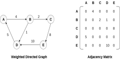
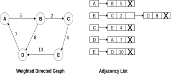
Representation of weighted directed graph is different. Instead of filling the entry by 1, the Non- zero entries of the adjacency matrix are represented by the weight of respective edges.

The weighted directed graph along with the adjacency matrix representation is shown in the following figure.

Linked Representation

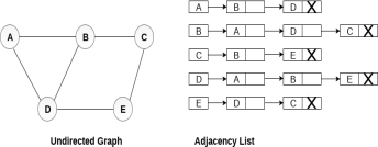
In the linked representation, an adjacency list is used to store the Graph into the computer's memory.

Consider the undirected graph shown in the following figure and check the adjacency list representation.

An adjacency list is maintained for each node present in the graph which stores the node value and a pointer to the next adjacent node to the respective node. If all the adjacent nodes are traversed then store the NULL in the pointer field of last node of the list. The sum of the lengths of adjacency lists is equal to the twice of the number of edges present in an undirected graph.

Consider the directed graph shown in the following figure and check the adjacency list representation of the graph.

In a directed graph, the sum of lengths of all the adjacency lists is equal to the number of edges present in the graph.

In the case of weighted directed graph, each node contains an extra field that is called the weight of the node. The adjacency list representation of a directed graph is shown in the following figure.

Q3) Explain path matrix.

A3)

The Floyd Warshall Algorithm is for solving the All Pairs Shortest Path problem. The problem is to find shortest distances between every pair of vertices in a given edge weighted directed Graph.

Floyd–Warshall algorithm is an algorithm for finding shortest paths in a weighted graph with positive or negative edge weights (but with no negative cycles).

A single execution of the algorithm will find the lengths (summed weights) of the shortest paths between all pairs of vertices.

Although it does not return details of the paths themselves, it is possible to reconstruct the paths with simple modifications to the algorithm.

#include<stdio.h>

#define MAX 100

void display(int matrix[MAX][MAX], int n);

int adj[MAX][MAX];

int n;

void create_graph();

int main()

{

        int i,j,k;

        int P[MAX][MAX];

        create_graph();

        printf("\nThe adjacency matrix is :\n");

        display(adj,n);

        for(i=0; i<n; i++)

           for(j=0; j<n; j++)

                 P[i][j] = adj[i][j];

        for(k=0; k<n; k++)

        {

                for(i=0; i<n; i++)

                  for(j=0; j<n; j++)

                      P[i][j] = ( P[i][j] || ( P[i][k] && P[k][j] ) );

                printf("\nP%d is :\n",k);

                display(P,n);

        }

        printf("\nP%d is the path matrix of the given graph\n",k-1);

}/*End of main() */

void display(int matrix[MAX][MAX],int n)

{

        int i,j;

        for(i=0; i<n; i++)

        {

                for(j=0; j<n; j++)

                        printf("%3d",matrix[i][j]);

                printf("\n");

        }

}/*End of display()*/

void create_graph()

{

        int i,max_edges,origin,destin;

        printf("\nEnter number of vertices : ");

        scanf("%d",&n);

        max_edges = n*(n-1);

        for( i=1; i<=max_edges; i++ )

        {

 printf("\nEnter edge %d( -1 -1 ) to quit : ",i);

                scanf("%d %d",&origin,&destin);

                if((origin == -1) && (destin == -1))

                        break;

                if( origin >= n || destin >= n || origin<0 || destin<0)

                {

                        printf("\nInvalid edge!\n");

                        i--;

                }

                else

                        adj[origin][destin] = 1;

        }/*End of for*/

}/*End of create_graph()*/

OUTPUT : :

/*  C Program to find Path Matrix by Warshall's Algorithm  */

Enter number of vertices : 4

Enter edge 1( -1 -1 ) to quit : 0 1

Enter edge 2( -1 -1 ) to quit : 0 2

Enter edge 3( -1 -1 ) to quit : 0 3

Enter edge 4( -1 -1 ) to quit : 1 3

Enter edge 5( -1 -1 ) to quit : 2 3

Enter edge 6( -1 -1 ) to quit : -1 -1

The adjacency matrix is :

  0  1  1  1

  0  0  0  1

  0  0  0  1

  0  0  0  0

P0 is :

  0  1  1  1

  0  0  0  1

  0  0  0  1

  0  0  0  0

P1 is :

  0  1  1  1

  0  0  0  1

  0  0  0  1

  0  0  0  0

P2 is :

  0  1  1  1

  0  0  0  1

  0  0  0  1

  0  0  0  0

P3 is :

  0  1  1  1

  0  0  0  1

  0  0  0  1

  0  0  0  0

P3 is the path matrix of the given graph

Process returned 0

Q4) What is BFS Algorithm (Breadth-First Search)? What are Graph traversals?

A4) Breadth-first search (BFS) is an algorithm that is used to graph data or searching tree or traversing structures. The full form of BFS is the Breadth-first search.

The algorithm efficiently visits and marks all the key nodes in a graph in an accurate breadthwise fashion. This algorithm selects a single node (initial or source point) in a graph and then visits all the nodes adjacent to the selected node. Remember, BFS accesses these nodes one by one.

Once the algorithm visits and marks the starting node, then it moves towards the nearest unvisited nodes and analyses them. Once visited, all nodes are marked. These iterations continue until all the nodes of the graph have been successfully visited and marked.

Graph traversals

A graph traversal is a commonly used methodology for locating the vertex position in the graph. It is an advanced search algorithm that can analyze the graph with speed and precision along with marking the sequence of the visited vertices. This process enables you to quickly visit each node in a graph without being locked in an infinite loop.

The architecture of BFS algorithm

Q5) Why do we need BFS Algorithm? How does BFS Algorithm Work?

A5) There are numerous reasons to utilize the BFS Algorithm to use as searching for your dataset. Some of the most vital aspects that make this algorithm your first choice is:

Graph traversal requires the algorithm to visit, check, and/or updates every single un-visited node in a tree-like structure. Graph traversals are categorized by the order in which they visit the nodes on the graph.

BFS algorithm starts the operation from the first or starting node in a graph and traverses it thoroughly. Once it successfully traverses the initial node, then the next non-traversed vertex in the graph is visited and marked.

Breadth first search is a graph traversal algorithm that starts traversing the graph from root node and explores all the neighbouring nodes. Then, it selects the nearest node and explore all the unexplored nodes. The algorithm follows the same process for each of the nearest node until it finds the goal.

The algorithm of breadth first search is given below. The algorithm starts with examining the node A and all of its neighbours. In the next step, the neighbours of the nearest node of A are explored and process continues in the further steps. The algorithm explores all neighbours of all the nodes and ensures that each node is visited exactly once and no node is visited twice.

Algorithm

Example

Consider the graph G shown in the following image, calculate the minimum path p from node A to node E. Given that each edge has a length of 1.

Solution:

Minimum Path P can be found by applying breadth first search algorithm that will begin at node A and will end at E. the algorithm uses two queues, namely QUEUE1 and QUEUE2. QUEUE1 holds all the nodes that are to be processed while QUEUE2 holds all the nodes that are processed and deleted from QUEUE1.

Let’s start examining the graph from Node A.

1. Add A to QUEUE1 and NULL to QUEUE2.

2. Delete the Node A from QUEUE1 and insert all its neighbours. Insert Node A into QUEUE2

3. Delete the node B from QUEUE1 and insert all its neighbours. Insert node B into QUEUE2.

4. Delete the node D from QUEUE1 and insert all its neighbours. Since F is the only neighbour of it which has been inserted, we will not insert it again. Insert node D into QUEUE2.

5. Delete the node C from QUEUE1 and insert all its neighbours. Add node C to QUEUE2.

6. Remove F from QUEUE1 and add all its neighbours. Since all of its neighbours has already been added, we will not add them again. Add node F to QUEUE2.

7. Remove E from QUEUE1, all of E's neighbours has already been added to QUEUE1 therefore we will not add them again. All the nodes are visited and the target node i.e. E is encountered into QUEUE2.

Now, backtrack from E to A, using the nodes available in QUEUE2.

The minimum path will be A → B → C → E.

Q6) What are the Rules and application of BFS Algorithm?

A6) Here, are important rules for using BFS algorithm:

Applications of BFS Algorithm

Let's take a look at some of the real-life applications where a BFS algorithm implementation can be highly effective.

Q7) Give a small brief on BFS algorithm

A7)

Q8) Explain DFS Algorithm.

A8) Depth first search (DFS) algorithm starts with the initial node of the graph G, and then goes to deeper and deeper until we find the goal node or the node which has no children. The algorithm, then backtracks from the dead end towards the most recent node that is yet to be completely unexplored.

The data structure which is being used in DFS is stack. The process is similar to BFS algorithm. In DFS, the edges that leads to an unvisited node are called discovery edges while the edges that leads to an already visited node are called block edges.

Algorithm

Example:

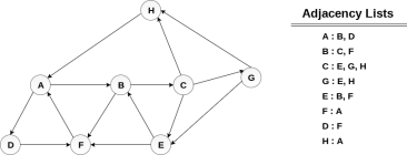
Consider the graph G along with its adjacency list, given in the figure below. Calculate the order to print all the nodes of the graph starting from node H, by using depth first search (DFS) algorithm.

Solution:

Push H onto the stack

POP the top element of the stack i.e. H, print it and push all the neighbours of H onto the stack that are is ready state.

Pop the top element of the stack i.e. A, print it and push all the neighbours of A onto the stack that are in ready state.

Pop the top element of the stack i.e. D, print it and push all the neighbours of D onto the stack that are in ready state.

Pop the top element of the stack i.e. F, print it and push all the neighbours of F onto the stack that are in ready state.

Pop the top of the stack i.e. B and push all the neighbours

Pop the top of the stack i.e. C and push all the neighbours.

Pop the top of the stack i.e. G and push all its neighbours.

Pop the top of the stack i.e. E and push all its neighbours.

Hence, the stack now becomes empty and all the nodes of the graph have been traversed.

The printing sequence of the graph will be :

Q9) Difference between BFS and DFS Binary Tree.

A9)

Q10) Explain Bellman Ford Algorithm

A10) This algorithm solves the single source shortest path problem of a directed graph G = (V, E) in which the edge weights may be negative. Moreover, this algorithm can be applied to find the shortest path, if there does not exist any negative weighted cycle.

Algorithm: Bellman-Ford-Algorithm (G, w, s)

for each vertex v Є G.V 

v.d := ∞

v.∏ := NIL

s.d := 0

for i = 1 to |G.V| - 1

for each edge (u, v) Є G.E

if v.d > u.d + w(u, v)

v.d := u.d +w(u, v)

v.∏ := u

for each edge (u, v) Є G.E

if v.d > u.d + w(u, v)

return FALSE

return TRUE

Analysis

The first for loop is used for initialization, which runs in O(V) times. The next for loop runs |V - 1| passes over the edges, which takes O(E) times.

Hence, Bellman-Ford algorithm runs in O(V, E) time.

Example

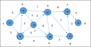
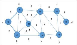
The following example shows how Bellman-Ford algorithm works step by step. This graph has a negative edge but does not have any negative cycle, hence the problem can be solved using this technique.

At the time of initialization, all the vertices except the source are marked by ∞ and the source is marked by 0.

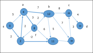
In the first step, all the vertices which are reachable from the source are updated by minimum cost. Hence, vertices a and h are updated.

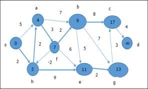
In the next step, vertices a, b, f and e are updated.

Following the same logic, in this step vertices b, f, c and g are updated.

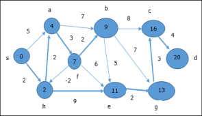
Here, vertices c and d are updated.

Hence, the minimum distance between vertex s and vertex d is 20.

Based on the predecessor information, the path is s→ h→ e→ g→ c→ d