undefined | unit 6 graphs

Unit VI

Graphs

What is graph and what is its terminology?

Graph

A graph can be defined as group of vertices and edges that are used to connect these vertices. A graph can be seen as a cyclic tree, where the vertices (Nodes) maintain any complex relationship among them instead of having parent child relationship.

Definition

A graph G can be defined as an ordered set G(V, E) where V(G) represents the set of vertices and E(G) represents the set of edges which are used to connect these vertices.

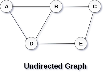
A Graph G(V, E) with 5 vertices (A, B, C, D, E) and six edges ((A,B), (B,C), (C,E), (E,D), (D,B), (D,A)) is shown in the following figure.

Graph

Directed and Undirected Graph

A graph can be directed or undirected. However, in an undirected graph, edges are not associated with the directions with them. An undirected graph is shown in the above figure since its edges are not attached with any of the directions. If an edge exists between vertex A and B then the vertices can be traversed from B to A as well as A to B.

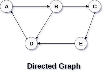
In a directed graph, edges form an ordered pair. Edges represent a specific path from some vertex A to another vertex B. Node A is called initial node while node B is called terminal node.

A directed graph is shown in the following figure.

Graph

Graph Terminology

Path

A path can be defined as the sequence of nodes that are followed in order to reach some terminal node V from the initial node U.

Closed Path

A path will be called as closed path if the initial node is same as terminal node. A path will be closed path if V0=VN.

Simple Path

If all the nodes of the graph are distinct with an exception V0=VN, then such path P is called as closed simple path.

Cycle

A cycle can be defined as the path which has no repeated edges or vertices except the first and last vertices.

Connected Graph

A connected graph is the one in which some path exists between every two vertices (u, v) in V. There are no isolated nodes in connected graph.

Complete Graph

A complete graph is the one in which every node is connected with all other nodes. A complete graph contain n(n-1)/2 edges where n is the number of nodes in the graph.

Weighted Graph

In a weighted graph, each edge is assigned with some data such as length or weight. The weight of an edge e can be given as w(e) which must be a positive (+) value indicating the cost of traversing the edge.

Digraph

A digraph is a directed graph in which each edge of the graph is associated with some direction and the traversing can be done only in the specified direction.

Loop

An edge that is associated with the similar end points can be called as Loop.

Adjacent Nodes

If two nodes u and v are connected via an edge e, then the nodes u and v are called as neighbours or adjacent nodes.

Degree of the Node

A degree of a node is the number of edges that are connected with that node. A node with degree 0 is called as isolated node.

2. What is Adjacency Matrix?

Adjacency matrix is a sequential representation.

It is used to represent which nodes are adjacent to each other. i.e. is there any edge connecting nodes to a graph.

In this representation, we have to construct a nXn matrix A. If there is any edge from a vertex i to vertex j, then the corresponding element of A, ai,j = 1, otherwise ai,j= 0.

Note, even if the graph on 100 vertices contains only 1 edge, we still have to have a 100x100 matrix with lots of zeroes.

If there is any weighted graph then instead of 1s and 0s, we can store the weight of the edge.

Example

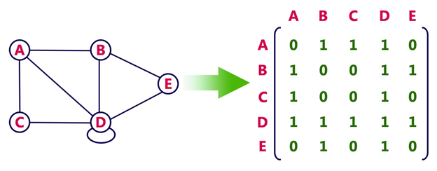
Consider the following undirected graph representation:

Undirected graph representation

Graph Representations

Directed graph represenation

See the directed graph representation:

Graph Representations

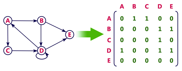
In the above examples, 1 represents an edge from row vertex to column vertex, and 0 represents no edge from row vertex to column vertex.

Undirected weighted graph represenation

Graph Representations

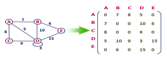
Pros: Representation is easier to implement and follow.

Cons: It takes a lot of space and time to visit all the neighbors of a vertex, we have to traverse all the vertices in the graph, which takes quite some time.

3. What is Incidence Matrix?

In Incidence matrix representation, graph can be represented using a matrix of size:

Total number of vertices by total number of edges.

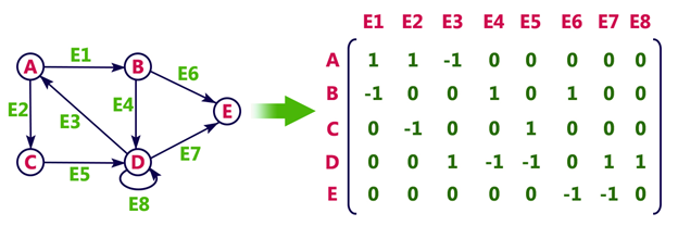
It means if a graph has 4 vertices and 6 edges, then it can be represented using a matrix of 4X6 class. In this matrix, columns represent edges and rows represent vertices.

This matrix is filled with either 0 or 1 or -1. Where,

0 is used to represent row edge which is not connected to column vertex.

1 is used to represent row edge which is connected as outgoing edge to column vertex.

-1 is used to represent row edge which is connected as incoming edge to column vertex.

Example

Consider the following directed graph representation.

Graph Representations

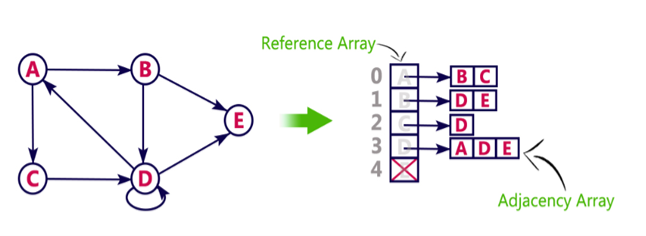
4. What is Adjacency List?

Adjacency list is a linked representation.

In this representation, for each vertex in the graph, we maintain the list of its neighbors. It means, every vertex of the graph contains list of its adjacent vertices.

We have an array of vertices which is indexed by the vertex number and for each vertex v, the corresponding array element points to a singly linked list of neighbors of v.

Example

Let's see the following directed graph representation implemented using linked list:

Graph Representations

We can also implement this representation using array as follows:

Graph Representations

Pros:

Adjacency list saves lot of space.

We can easily insert or delete as we use linked list.

Such kind of representation is easy to follow and clearly shows the adjacent nodes of node.

Cons:

The adjacency list allows testing whether two vertices are adjacent to each other but it is slower to support this operation.

5. Explain Data Structure - Depth First Traversal

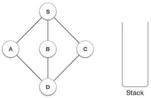
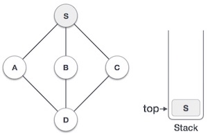
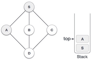
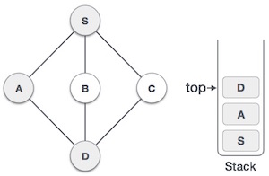
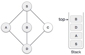
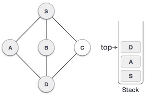
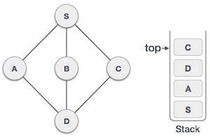
Depth First Search (DFS) algorithm traverses a graph in a depthward motion and uses a stack to remember to get the next vertex to start a search, when a dead end occurs in any iteration.

Depth First Travesal

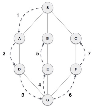
As in the example given above, DFS algorithm traverses from S to A to D to G to E to B first, then to F and lastly to C. It employs the following rules.

Rule 1 − Visit the adjacent unvisited vertex. Mark it as visited. Display it. Push it in a stack.

Rule 2 − If no adjacent vertex is found, pop up a vertex from the stack. (It will pop up all the vertices from the stack, which do not have adjacent vertices.)

Rule 3 − Repeat Rule 1 and Rule 2 until the stack is empty.

Step	Traversal	Description
1		Initialize the stack.
2		Mark S as visited and put it onto the stack. Explore any unvisited adjacent node from S. We have three nodes and we can pick any of them. For this example, we shall take the node in an alphabetical order.
3		Mark A as visited and put it onto the stack. Explore any unvisited adjacent node from A. Both S and D are adjacent to A but we are concerned for unvisited nodes only.
4		Visit D and mark it as visited and put onto the stack. Here, we have B and C nodes, which are adjacent to D and both are unvisited. However, we shall again choose in an alphabetical order.
5		We choose B, mark it as visited and put onto the stack. Here B does not have any unvisited adjacent node. So, we pop B from the stack.
6		We check the stack top for return to the previous node and check if it has any unvisited nodes. Here, we find D to be on the top of the stack.
7		Only unvisited adjacent node is from D is C now. So we visit C, mark it as visited and put it onto the stack.

As C does not have any unvisited adjacent node so we keep popping the stack until we find a node that has an unvisited adjacent node. In this case, there's none and we keep popping until the stack is empty.

6. Explain Data Structure - Breadth First Traversal

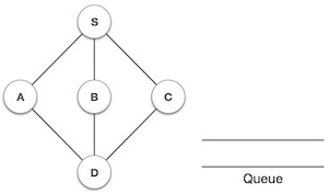
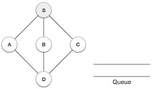
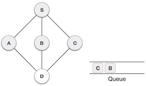
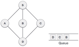
Breadth First Search (BFS) algorithm traverses a graph in a breadthward motion and uses a queue to remember to get the next vertex to start a search, when a dead end occurs in any iteration.

Breadth First Traversal

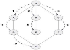
As in the example given above, BFS algorithm traverses from A to B to E to F first then to C and G lastly to D. It employs the following rules.

Rule 1 − Visit the adjacent unvisited vertex. Mark it as visited. Display it. Insert it in a queue.

Rule 2 − If no adjacent vertex is found, remove the first vertex from the queue.

Rule 3 − Repeat Rule 1 and Rule 2 until the queue is empty.

Step	Traversal	Description
1		Initialize the queue.
2		We start from visiting S (starting node), and mark it as visited.
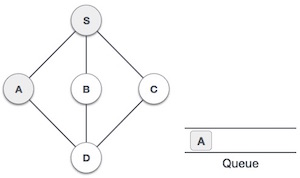
3		We then see an unvisited adjacent node from S. In this example, we have three nodes but alphabetically we choose A, mark it as visited and enqueue it.
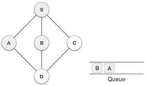
4		Next, the unvisited adjacent node from S is B. We mark it as visited and enqueue it.
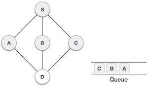
5		Next, the unvisited adjacent node from S is C. We mark it as visited and enqueue it.
6		Now, S is left with no unvisited adjacent nodes. So, we dequeue and find A.
7		From A we have D as unvisited adjacent node. We mark it as visited and enqueue it.

At this stage, we are left with no unmarked (unvisited) nodes. But as per the algorithm we keep on dequeuing in order to get all unvisited nodes. When the queue gets emptied, the program is over.

7. Explain Spanning Tree

A spanning tree is a subset of Graph G, which has all the vertices covered with minimum possible number of edges. Hence, a spanning tree does not have cycles and it cannot be disconnected..

By this definition, we can draw a conclusion that every connected and undirected Graph G has at least one spanning tree. A disconnected graph does not have any spanning tree, as it cannot be spanned to all its vertices.

Spanning Trees

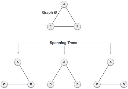
We found three spanning trees off one complete graph. A complete undirected graph can have maximum nn-2 number of spanning trees, where n is the number of nodes. In the above addressed example, n is 3, hence 33−2 = 3 spanning trees are possible.

General Properties of Spanning Tree

We now understand that one graph can have more than one spanning tree. Following are a few properties of the spanning tree connected to graph G −

A connected graph G can have more than one spanning tree.

All possible spanning trees of graph G, have the same number of edges and vertices.

The spanning tree does not have any cycle (loops).

Removing one edge from the spanning tree will make the graph disconnected, i.e. the spanning tree is minimally connected.

Adding one edge to the spanning tree will create a circuit or loop, i.e. the spanning tree is maximally acyclic.

Mathematical Properties of Spanning Tree

Spanning tree has n-1 edges, where n is the number of nodes (vertices).

From a complete graph, by removing maximum e - n + 1 edges, we can construct a spanning tree.

A complete graph can have maximum nn-2 number of spanning trees.

Thus, we can conclude that spanning trees are a subset of connected Graph G and disconnected graphs do not have spanning tree.

Application of Spanning Tree

Spanning tree is basically used to find a minimum path to connect all nodes in a graph. Common application of spanning trees are −

Civil Network Planning

Computer Network Routing Protocol

Cluster Analysis

Let us understand this through a small example. Consider, city network as a huge graph and now plans to deploy telephone lines in such a way that in minimum lines we can connect to all city nodes. This is where the spanning tree comes into picture.

Minimum Spanning Tree (MST)

In a weighted graph, a minimum spanning tree is a spanning tree that has minimum weight than all other spanning trees of the same graph. In real-world situations, this weight can be measured as distance, congestion, traffic load or any arbitrary value denoted to the edges.

8. What is Kruskal's Spanning Tree

Kruskal's algorithm to find the minimum cost spanning tree uses the greedy approach. This algorithm treats the graph as a forest and every node it has as an individual tree. A tree connects to another only and only if, it has the least cost among all available options and does not violate MST properties.

To understand Kruskal's algorithm let us consider the following example −

MST Graph

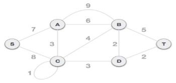
Step 1 - Remove all loops and Parallel Edges

Remove all loops and parallel edges from the given graph.

MST Graph with loops

In case of parallel edges, keep the one which has the least cost associated and remove all others.

MST Graph without loops

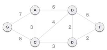
Step 2 - Arrange all edges in their increasing order of weight

The next step is to create a set of edges and weight, and arrange them in an ascending order of weightage (cost).

MST ascending weightage

Step 3 - Add the edge which has the least weightage

Now we start adding edges to the graph beginning from the one which has the least weight. Throughout, we shall keep checking that the spanning properties remain intact. In case, by adding one edge, the spanning tree property does not hold then we shall consider not to include the edge in the graph.

MST Graph step one

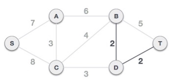
The least cost is 2 and edges involved are B,D and D,T. We add them. Adding them does not violate spanning tree properties, so we continue to our next edge selection.

Next cost is 3, and associated edges are A,C and C,D. We add them again −

MST Graph step two

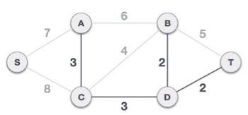
Next cost in the table is 4, and we observe that adding it will create a circuit in the graph. −

MST Graph step three

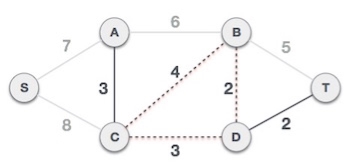
We ignore it. In the process we shall ignore/avoid all edges that create a circuit.

MST Graph step four

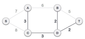
We observe that edges with cost 5 and 6 also create circuits. We ignore them and move on.

MST Graph step five

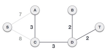
Now we are left with only one node to be added. Between the two least cost edges available 7 and 8, we shall add the edge with cost 7.

MST Kruskals Algorithm

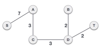
By adding edge S,A we have included all the nodes of the graph and we now have minimum cost spanning tree.

9. What is Prim's Spanning Tree?

Prim's algorithm to find minimum cost spanning tree (as Kruskal's algorithm) uses the greedy approach. Prim's algorithm shares a similarity with the shortest path first algorithms.

Prim's algorithm, in contrast with Kruskal's algorithm, treats the nodes as a single tree and keeps on adding new nodes to the spanning tree from the given graph.

To contrast with Kruskal's algorithm and to understand Prim's algorithm better, we shall use the same example −

MST Graph

Step 1 - Remove all loops and parallel edges

MST Graph with loops

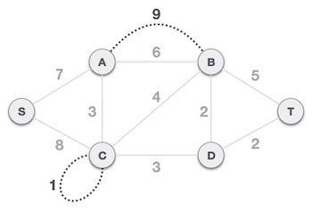
Remove all loops and parallel edges from the given graph. In case of parallel edges, keep the one which has the least cost associated and remove all others.

MST Graph without loops

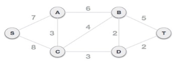
Step 2 - Choose any arbitrary node as root node

In this case, we choose S node as the root node of Prim's spanning tree. This node is arbitrarily chosen, so any node can be the root node. One may wonder why any video can be a root node. So the answer is, in the spanning tree all the nodes of a graph are included and because it is connected then there must be at least one edge, which will join it to the rest of the tree.

Step 3 - Check outgoing edges and select the one with less cost

After choosing the root node S, we see that S,A and S,C are two edges with weight 7 and 8, respectively. We choose the edge S,A as it is lesser than the other.

MST Graph Step 1

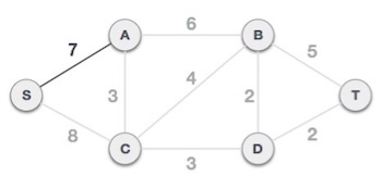
Now, the tree S-7-A is treated as one node and we check for all edges going out from it. We select the one which has the lowest cost and include it in the tree.

MST Graph Step 2

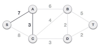
After this step, S-7-A-3-C tree is formed. Now we'll again treat it as a node and will check all the edges again. However, we will choose only the least cost edge. In this case, C-3-D is the new edge, which is less than other edges' cost 8, 6, 4, etc.

MST Graph Step 3

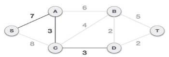
After adding node D to the spanning tree, we now have two edges going out of it having the same cost, i.e. D-2-T and D-2-B. Thus, we can add either one. But the next step will again yield edge 2 as the least cost. Hence, we are showing a spanning tree with both edges included.

MST Prim's Algorithm

We may find that the output spanning tree of the same graph using two different algorithms is same.

10. What is Dijkstra's Algorithm?

Dijkstra's algorithm has many variants but the most common one is to find the shortest paths from the source vertex to all other vertices in the graph.

Algorithm Steps:

Set all vertices distances = infinity except for the source vertex, set the source distance =

Push the source vertex in a min-priority queue in the form (distance , vertex), as the comparison in the min-priority queue will be according to vertices distances.

Pop the vertex with the minimum distance from the priority queue (at first the popped vertex = source).

Update the distances of the connected vertices to the popped vertex in case of "current vertex distance + edge weight < next vertex distance", then push the vertex
with the new distance to the priority queue.

If the popped vertex is visited before, just continue without using it.

Apply the same algorithm again until the priority queue is empty.

Implementation:

Assume the source vertex =

#define SIZE 100000 + 1

vector < pair < int , int > > v [SIZE]; // each vertex has all the connected vertices with the edges weights

int dist [SIZE];

bool vis [SIZE];

void dijkstra(){

// set the vertices distances as infinity

memset(vis, false , sizeof vis); // set all vertex as unvisited

dist[1] = 0;

multiset < pair < int , int > > s; // multiset do the job as a min-priority queue

s.insert({0 , 1}); // insert the source node with distance = 0

while(!s.empty()){

pair <int , int> p = *s.begin(); // pop the vertex with the minimum distance

s.erase(s.begin());

int x = p.s; int wei = p.f;

if( vis[x] ) continue; // check if the popped vertex is visited before

vis[x] = true;

for(int i = 0; i < v[x].size(); i++){

int e = v[x][i].f; int w = v[x][i].s;

if(dist[x] + w < dist[e] ){ // check if the next vertex distance could be minimized

dist[e] = dist[x] + w;

s.insert({dist[e], e} ); // insert the next vertex with the updated distance

}

Time Complexity of Dijkstra's Algorithm is

but with min-priority queue it drops down to

However, if we have to find the shortest path between all pairs of vertices, both of the above methods would be expensive in terms of time. Discussed below is another alogorithm designed for this case.

Sign Up