Unit 2

Curves and Surfaces

Q1) Explain the non-parametric representation of curves

A1) Non-parametric or Cartesian representation

For a nonparametric curve, the coordinates y and z of a point on the curve are expressed as two separate functions of the third coordinate x as the independent variable.

In other words, in non-parametric or cartesian system, the curve is represented as a relation between the coordinates x, y, z.

There are two forms of non-parametric representation of curves:

In explicit representation, coordinates are expressed as a function of any one independent coordinate.

Explicit Non-parametric representation for 2D curve is

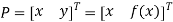
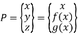
Explicit Non-parametric representation for 3D curve is

b.     Implicit representation

In implicit representation, the curve is represented as a relation between the coordinates.

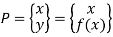
Implicit Non-parametric representation for 2D curve is

Implicit Non-parametric representation for 2D curve is

      Limitation of non-parametric or cartesian or generic representation of curves:

Q2) Explain Parametric Representation of Curves

A2)

All the difficulties in non-parametric representation are overcome in  parametric representation.

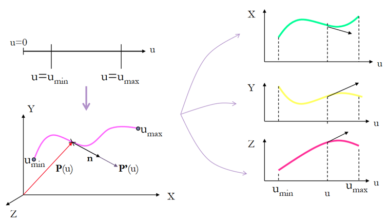
In parametric form, each point on a curve is expressed as a function of a parameter u.

Here, the coordinates are not in relation with each other but are the function of an independent parameter u [f(u)].

This independent coordinate acts as a local coordinate for the points on the curve.

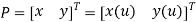
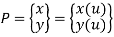
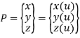
Parametric representation for 2D curve is

Where,

Parametric representation for 2D curve in matrix form is

Where,

The tangent vector at point P is

Parametric representation for 3D curve is

Where,

Parametric representation for 2D curve in matrix form is

Where,

The tangent vector at point P is

Q3) Explain C0, C1 and C2 continuity

A3) If each section of a spline is described with a set of parametric coordinate functions of the form

Where,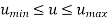

Zero-order parametric continuity, described as C0 continuity, means simply that the curves meet.

The end points of the two curve segments meet with each other in C0 continuity.

Zero-order continuity C0 yields a position continuous curve.

That is, the values of x, y, and z evaluated at u, for the first curve section are equal, respectively, to the values of x, y, and z evaluated at u, for the next curve section.

Mathematically,

(x, y, z for curve segment 1 at u = umax) = (x, y, z for curve segment 2 at u = umin)

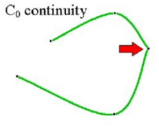
2.     First order continuity C1

First-order parametric continuity, C1 continuity, means that the first parametric derivatives (tangent lines) of the coordinate functions for two successive curve sections are equal at their joining point.

C1 continuity imply slope continuous curves

At the joining of two segments, the tangent or first order derivative of parametric equation of both curve segment coincides or are equal.

Mathematically,

(x’, y’, z’ for curve segment 1 at u = umax) = (x’, y’, z’ for curve segment 2 at u = umin)

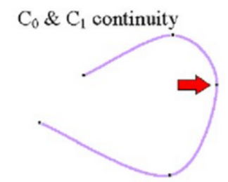
3.     Second Order Continuity C2

Second-order parametric continuity, or C2 continuity, means that both the first and second parametric derivatives of the two curve sections are the same at the intersection.

C2-order continuity imply curvature continuous curves.

At the joining of two segments, first order derivative as well as second order derivative of parametric equation of both curve segment coincides or are equal.

Mathematically,

(x’’, y’’, z’’ for curve segment 1 at u = umax) = (x’’, y’’, z’’ for curve segment 2 at u = umin)

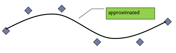
Q4) Explain need of synthetic curve and approaches to generate a synthetic curve

A4) Need of Synthetic curve

There are two approaches to generate synthetic curve

In interpolation, the curve passes through all the data points.

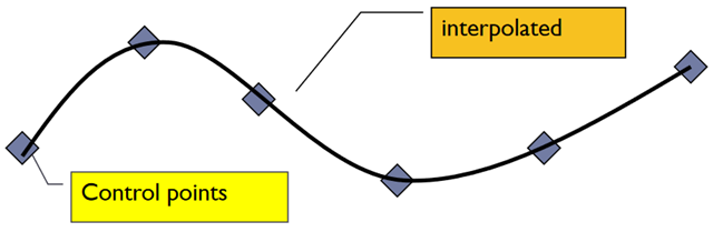
In approximation, curve does not pass through all data points but are close to data points.

Q5) Explain Bezier curve and give its characteristics

A5) “The Bezier curves uses the given data points for generating the curve and passes through first and last data points while other acts as control points.”

Bezier curves are used more than hermite cubic splines because of its flexibility to change shape of curve.

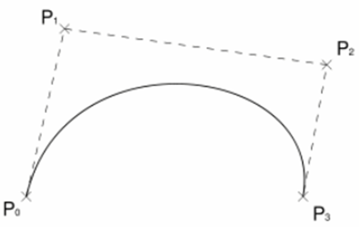
Bezier curve

Parametric equation of Bezier curve is written as,

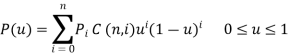
Or

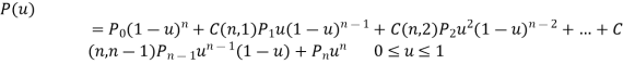
Where

Bezier curve for n+1 data point is nth degree polynomial.

Characteristics of Bezier curve

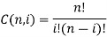
Q6) Give properties of NURBS curve

A6) Properties of NURBS curve

Q7) Derive the expression for Coons patch surface

A7) The corner points are blended in a bilinear surface, but four boundary curves are blended to form a surface in a Coon's patch. The word patch is used to indicate explicitly that the surface being generated is a surface segment corresponding to the parameter region . Thus, any arbitrary surface is composed by many of these patches.

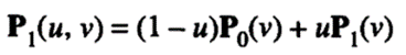
The equation of a Coon's patch is derived as follows. We assume that the equations of the four boundary curves are given by P0(v), P1(v), 'Q0(u), and Q1(u), as illustrated in Figure.

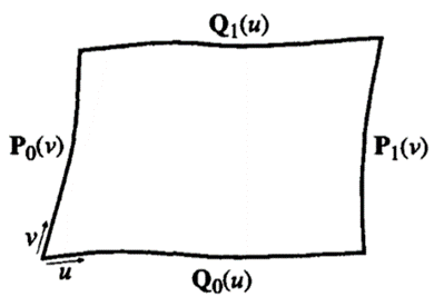
We also assume that the curves 'lo(u) and Q1(u) have the interval of u from 0 to 1 and the same direction. In Figure, we assume that their direction is to the right, as indicated by the arrow for u. Similarly, P0(v) and P1(v) have the interval of v from 0 to 1 and the same direction, upward in this case.

First, two curves facing each other are selected, say, P0(v) and P1 (v). Then they are interpolated in the u direction by a linear equation:

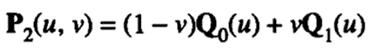
Now let's try to define another surface by interpolating Q0(u) and Q1(u) in the v direction:

Now, let's try yet another surface, P3(u, v), defined by adding P1(u, v) and P2(u, v) to determine whether it can be bounded by all the boundary curves. Then P3(u, v) becomes

and substituting the limit values of u and v

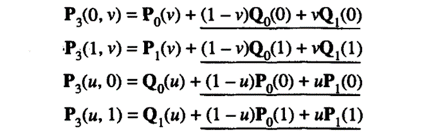
Each underlined term is the linear interpolation between the end points of the corresponding boundary curve. In other words, the terms to be eliminated are the expressions of the boundary curves of a bilinear surface

Therefore, the correct equation of a Coon's patch is obtained by subtracting the bilinear surface equation from P 3(u, v):

Q8) Write a note on Reverse Engineering

A8) Reverse engineering is the process of obtaining a geometric CAD model from measurements acquired by scanning an existing physical model. The measurements are in the form of 3D point clouds that correspond to points on the surface of the object being re-engineered. Using CAD models to represent the scanned object is very important in various industries because they help improve the quality and efficiency of design. In addition, they speed up the manufacturing and analysis process.

Reverse Engineering Methodology

The characterized typical procedure of reverse engineering shown in figure.

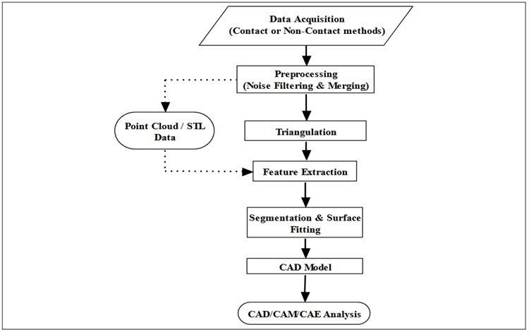
Reverse Engineering: It consists of five steps: (1) data acquisition, (2) preprocessing (noise filtering and merging), (3) triangulation, (4) feature extraction, and (5) segmentation and surface fitting. Data acquisition and processing systems includes hardware and software components. A hardware system acquires point clouds or volumetric data by using available experimental setup. A software system processes raw point clouds or volumetric data and transfers them into a virtual representation of object surfaces. The point cloud data is acquired in the form of x, y and z co-ordinates of the multiple point of the object surface. The scanning techniques use to scan the object are contact and noncontact technique.3D digitization system such as non-contact 3D scanner generated the large amount of data. In general, scanning data can be saved in different file formats, out of which the point cloud and STL formats are very useful for research assessment.

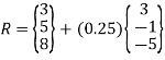
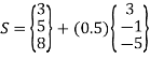
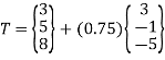
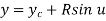
Q9) Write equation of line having end points P1(3,5,8) and P2(6,4,3). Find the tangent vector and coordinates of points on line at u=0.25,0.5,0.75.

A9)

P1(3,5,8) P2(6,4,3)

Parametric equation of ine:

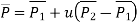
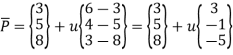
This is the equation of line.

Tangent vector of line:

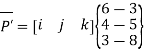
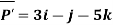
Coordinates of point:

At u = 0.25

At u = 0.5

At u = 0.75

The coordinates of points at

u = 0.25 is R(3.75,4.75,6.75)

u = 0.5 is S(4.5,4.5,5.5)

u = 0.75 is T(5.25,4.25,4.25)

Q10) A circle is represented by centre point (5,5) and radius 6 units. Find the parametric equation of circle and determine the various points on the circle in first quadrant if increment of angle is 45o and 90o.

A10)

Pc (xc, yc, zc) = (5,5,0)

Parametric equation of circle is given by

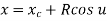
Where,

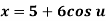
Where,

Coordinates of points on circle are given in table:

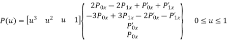
Q11)Calculate the points on Hermite cubic spline curve at u = 0, 0.2, 0.4, 0.6, 0.8 having end points P0 (4,4) and P1 (8,5). The tangent vector for ends P0 and P1 defined by line between P0 and P2 (5,6) and line between P1 and P3 (10,7).

A11)

P0 (4,4)  P1 (8,5) P2 (5,6) P3 (10,7)

Equation for x-coordinate:

P0x = 4 P1x = 8 P2x = 5 P3x = 10

Slope of tangent is given by

P’0x = P2x – P0x = 5 – 4 = 1

P’1x = P3x – P1x = 10 – 8 = 2

parametric equation of hermite curve for x-coordinate passing through two points P0 and P1 and two tangent vectors at these points P0’ and P1’ respectively is

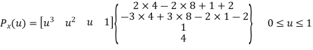
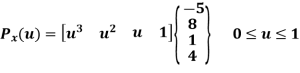
Equation for y-coordinate:

P0y = 4 P1y = 5 P2y = 6 P3y = 7

Slope of tangent is given by

P’0y = P2y – P0y = 6 – 4 = 2

P’1y = P3y – P1y = 7 – 5 = 2

General parametric equation of hermite curve passing through two points P0 and P1 and two tangent vectors at these points P0’ and P1’ respectively is

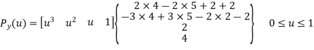
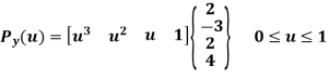
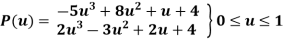
The parametric equation for hermite cubic spline is

Points on the hermite cubic spline are given in table