Unit - 3

Numerical Integration

Q1) What is trapezoidal rule?

A1)

Let the interval be divided into n equal intervals such that <<…. <=b.

Here.

To find the value of.

Setting n=1, we get

Or I =

The above is known as Trapezoidal method.

Q2) Compute the value of   ?

A2)

Using the trapezoidal rule with h=0.5, 0.25 and 0.125.

Here

For h=0.5, we construct the data table:

By Trapezoidal rule

For h=0.25, we construct the data table:

By Trapezoidal rule

For h = 0.125, we construct the data table:

By Trapezoidal rule

[(1+0.5) +2(0.98461+0.94117+0.87671+0.8+0.71910+0.64+0.56637)]

Q3) Evaluate, using trapezoidal rule with five ordinates

A3)

Here

We construct the data table:

X	0
Y	0	0.3693161	1.195328	1.7926992	1.477265	0

Q4) What do you understand by Simpson’s 1/3rd rule?

A4)

Let the interval be divided into n equal intervals such that <<…. <=b.

Here.

To find the value of.

Setting n = 2,

Which is known as Simpson’s 1/3- rule or Simpson’s rule.

Note: In this rule third and higher differences are neglected a so f(x) is a polynomial of degree 2.

Q5) Estimate the value of the integral

By Simpson’s rule with 4 strips and 8 strips respectively.

A5)

For n=4, we have

Construct the data table:

By Simpson’s Rule

For n = 8, we have

By Simpson’s Rule

Q6) Evaluate

A6)

Using Simpson’s 1/3 rule with .

For , we construct the data table:

X	0
	0	0.50874	0.707106	0.840896	0.930604	0.98281	1

By Simpson’s Rule

Q7) Evaluate By Simpson’s 3/8 rule.

A7)

Let us divide the range of the interval [4, 5.2] into six equal parts.

For h=0.2, we construct the data table:

X	4.0	4.2	4.4	4.6	4.8	5.0	5.2
	1.3863	1.4351	1.4816	1.5261	1.5686	1.6094	1.6487

By Simpson’s 3/8 rule

= 1.8278475

Q8) Evaluate

A8)

Let us divide the range of the interval [0,6] into six equal parts.

For h=1, we construct the data table:

X	0	1	2	3	4	5	6
	1	0.5	0.2	0.1	0.0588	0.0385	0.027

By Simpson’s 3/8 rule

+3(0.0385) +0.027]

=1.3571

Q9) Evaluate

A9)

Here

Using =

Also

For

For

Hence

Here

By Gauss quadrature 3-point rule

Q10) Evaluate  by 2-point Gaussian rule.

A10)

Here

Using =

Also

For

For

Hence

Here

By Gauss quadrature 2-point rule

=0.99847

Q11) Solve by Gauss quadrature 3-point method

A11)

Given

Here

Using =

Also

For

For

Hence

Here

By Gauss quadrature 3-point rule

Hence

Q12) Evaluate

A12)

Let

Here the interval of x and y are and .

Let 

Consider the following table:

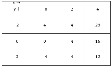
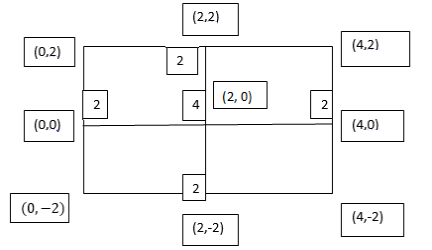
By Trapezoidal Rule

.

Q13) Evaluate 

A13)

Let

Here

Let the number of intervals be .

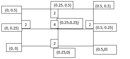
By Trapezoidal Rule

.

Q14) Evaluate

A14)

Let 

And

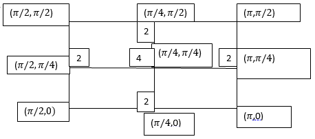
By Trapezoidal Rule

Q15) Evaluate 

A15)

Let

Here the interval of x and y are and .

Let 

Consider the following table:

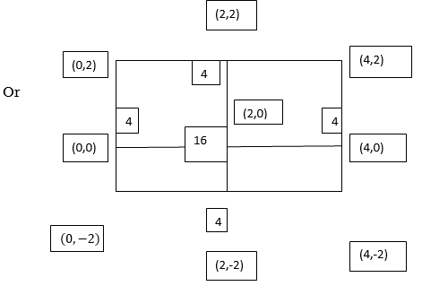
By Simpson’s 1/3 Rule

.4444444

Q16) Evaluate 

A16)

Let

Here

Let the number of intervals be .

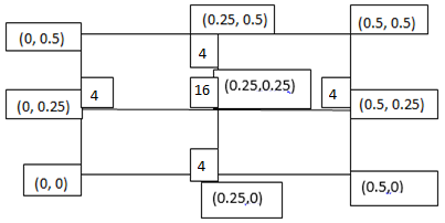
By Simpson’s 1/3 Rule

Q17) Evaluate

A17)

Let 

And

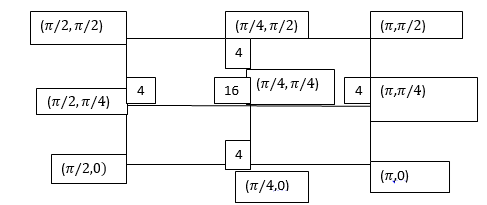
By Simpson’s 1/3 Rule