Unit - 5

Statistics

Q1) Find the mean of the following:

A1)

Q2) Find the arithmetic mean for the following distribution:

A2)

Let assumed mean

Class	Mid-value	Frequency
0-10 10-20 20-30 30-40 40-50	5 15 25 35 45	7 8 20 10 5	-20 -10 0 10 5	-140 -80 0 100 100
Total			50	-20

Q3) Find the value of Median from the following data.

A3)

The given cumulative frequency distribution will first be converted into ordinary frequency as under

Class Interval	Cumulative frequency	Ordinary frequency
0-5 5-10 15-20 20-25 25-35 30-35 35-40 40-45	29 465 582 634 644 650 653 655	29=29 224-29=195 465-224= 582-465=117 634-582=52 644-634=10 650-644=6 653-650=3 655-653=2

Median= size of or 327.5th item

327.5th item lies in 10-15 which is the median class.

Where stands for lower limit of median class,

N stands for the total frequency,

C stands for the cumulative frequency just preceding the median class,

stands for class interval

stands for frequency for the median class.

Median

Q4) Find the mode from the following data:

A4)

Age	Frequency	Cumulative frequency
Age	Frequency	Cumulative frequency
0-6 6-12 12-18 24-30 30-36 36-42	6 11 25 35 12 6	6 17 42 77 95 107 113

Mode

Q5) Compute the variance and standard deviation.

A5)

Class	Mid-value (x)	Frequency (f)
0-10	5	3	1470.924
10-20	15	5	737.250
20-30	25	7	32.1441
30-40	35	9	555.606
40-50	45	4	1275.504
Sum			4071.428

Then standard deviation,

Q6) Calculate S.D for the following distribution.

A6)

Wages earned C.I	Mid value	Frequency
52	5	5	-2	-10	20
153	15	9	-1	-9	9
25	25	15	0	0	0
35	35	12	1	12	12
45	45	10	2	20	40
55	55	3	3	9	27
Total	-

Using formula,

Q7) Calculate coefficient variation for the following frequency distribution.

A7)

We already calculated

Now, 

A.M    

A.M    

Coefficient of Variation

Q8) What do you understand by standard error?

A8)

Standard deviation and standard error of the mean are both statistical measures of variability. While the standard deviation of a sample depicts the spread of observations within the given sample regardless of the population mean, the standard error of the mean measures the degree of dispersion of sample means around the population mean.

The standard error is calculated as

is the standard deviation and n is the sample size.

Q9) Find the quartile deviation of the following data-

A9)

Here N/4 = 28/4 = 7 so that the 7’th observation falls in class 10 – 20.

And

3N/4 = 21, and 21’st observation falls in the interval 30 – 40 which is the third quartile.

The quartiles can be calculated as below-

And

Hence the quartile deviation is-

Q10) Explain skewness and kurtosis.

A10)

Skewness denotes the opposite of symmetry. It is lack of symmetry. In a symmetrical series, the mode, the median, and the arithmetic average are identical.

Coefficient of skewness

KURTOSIS: It measures the degree of peakedness of a distribution and is given by Measure of kurtosis.

Negative skewness      Positive skewness A: Mesokurtic B: Leptokurtic

C: Playkurtic

If , the curve is normal or mesokurtic.

If , the curve is peaked or leptokurtic.

If , the curve is flat topped or platykurtic

Q11) Calculate the median, quartiles and the quartile coefficient of skewness from the following data:

A11)

Here total frequency =230

The cumulative frequency table is

Weight (lbs)	70-80	80-90	90-100	100-110	110-120	120-130	130-140	140-150
	12	18	35	42	50	45	20	8
	12	30	65	107	157	202	222	230

Now item which lies in 110-120 group.

 Median or

Also i.e., is or item which lies in 90-100 group.

Similarly, i.e.,is item which lies in 120-130 group.

Hence quartile coefficient of skewness

(approx)

Q12) Explain correlation.

A12)

When two variables are related in such a way that a change in the value of one variable affects the value of the other variable, then these two variables are said to be correlated and there is a correlation between two variables.

Example- Height and weight of the persons of a group.

The correlation is said to be a perfect correlation if two variables vary in such a way that their ratio is constant always.

Basically, correlation is the measurement of the strength of a linear relationship between two variables.

In other words, we define the correlation as- if the change in one variable affects a change in other variable, then these two variables are said to be correlated.

For example:

1. The correlation between a person’s income and expenditures.
2. As the temperature goes up, the demand of ice cream also goes up.

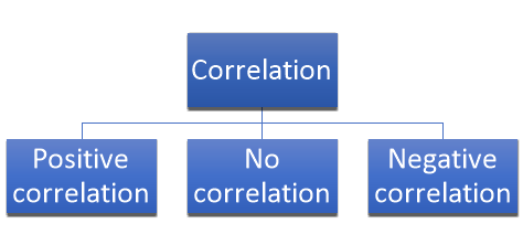
Types of correlation

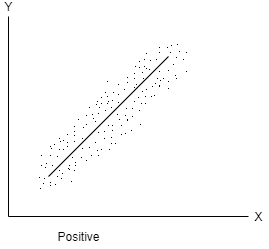
Positive correlation- When both variables move in the same direction, or if the increase in one variable results in a corresponding increase in the other one is called positive correlation.

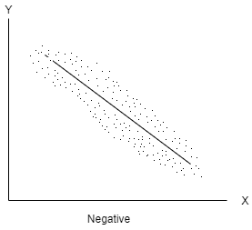
Negative correlation- When one variable increases and other decreases or vice-versa, then the variables said to be negatively correlated.

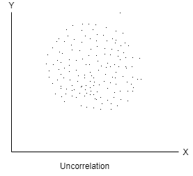
No correlation- When two variables are independent and do not affect each other then there will be no correlation between the two and said to be un-correlated.

Note- (Perfect correlation)- When a variable changes constantly with the other variable, then these two variables are said to be perfectly correlated.

Q13) What is the Karl Pearson coefficient of correlation?

A13)

Karl Pearson’s coefficient of correlation-

Here- and

Note-

1. Correlation coefficient always lies between -1 and +1.

2. Correlation coefficient is independent of the change of origin and scale.

3. If the two variables are independent then the correlation coefficient between them is zero.

Q14) Find the correlation coefficient between age and weight of the following data-

A14)

x	y					( ) )
30	56	-10	100	-4	16	40
44	55	4	16	-5	25	-20
45	60	5	25	0	0	0
43	64	3	9	4	16	12
34	62	-6	36	2	4	-12
44	63	4	16	3	9	12
Sum= 240	360	0	202	0	70	32

Karl Pearson’s coefficient of correlation-

Q15) Find the correlation coefficient between the values X and Y of the dataset given below by using the short-cut method-

A15)

X	Y
10	90	-20	400	20	400	-400
20	85	-10	100	15	225	-150
30	80	0	0	10	100	0
40	60	10	100	-10	100	-100
50	45	20	400	-25	625	-500
Sum = 150	360	0	1000	10	1450	-1150

Short-cut method to calculate correlation coefficient-

Q16) Derive the rank correlation formula.

A16)

Let be the ranks of the ith individuals in A and B respectively. Assuming that no two individuals are bracketed equal in either case, each of the variables taking the values 1,2, 3…, n we have

If X, Y be the deviations of x, y from their means, then

Now let,

Hence the correlation coefficient between these variables is

This is called the rank correlation coefficient and is denoted by

Q17) Three judges A, B, C give the following ranks. Find which pair of judges has common approach

A17)

Here n = 10

A (=x)	Ranks by B(=y)	C (=z)	x-y	y - z	z-x
1	3	6	-2	-3	5	4	9	25
6	5	4	1	1	-2	1	1	4
5	8	9	-3	-1	4	9	1	16
10	4	8	6	-4	-2	36	16	4
3	7	1	-4	6	-2	16	36	4
2	10	2	-8	8	0	64	64	0
4	2	3	2	-1	-1	4	1	1
9	1	10	8	-9	1	64	81	1
7	6	5	1	1	-2	1	1	4
8	9	7	-1	2	-1	1	4	1
Total			0	0	0	200	214	60

Since is maximum, the pair of judge A and C have the nearest common approach.

Q18) If X and Y are uncorrelated random variables, the of correlation between and

A18)

Let and

Then

Now

Similarly,

Now

Also

(As and are not correlated, we have )

Similarly,