Unit - 2

Structured Query Language (SQL)

Q1) Explain the sql data types?

A1) 

SQL data types

In order to describe the values that a column can hold, SQL Datatype is used.

Each column is needed in the database table to have a name and data type.

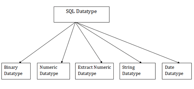
Fig 1: SQL data types

1. Binary data types

Three kinds of binary data types are given below:

2.     Numeric data types

The subtypes are given below:

3.     Extract numeric data types

The subtypes are given below:

4.     Character String data types

5.     Date and Time data types

Q2) What is the primary key?

A2) Primary key

The primary key is a field that uniquely identifies each table row. If a column in a table is designated as a primary key, it cannot include NULL values, and all rows must have unique values for this field. To put it another way, this is a combination of NOT NULL and UNIQUE constraints.

CREATE TABLE STUDENT(

ROLL_NO   INT  NOT NULL,

STU_NAME VARCHAR (35)  NOT NULL UNIQUE,

STU_AGE INT NOT NULL,

STU_ADDRESS VARCHAR (35) UNIQUE,

PRIMARY KEY (ROLL_NO)

);

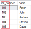
The ROLL NO field is marked as primary key in the example below, which means it cannot contain duplicate or null entries.

Q3) Define foreign key?

A3) Foreign key

A foreign key differs from a super key, candidate key, or primary key in that it is used to join two tables or link them together.

A foreign key is a secondary key that connects two tables via the primary key. It signifies that one table's columns point to the other table's primary key attribute. It also means that any attribute set as a primary key attribute will serve as a foreign key attribute in another table. A foreign key, on the other hand, has nothing to do with the primary key.

A Foreign Key column establishes a connection between two tables. Foreign keys are used to guarantee data integrity while also allowing navigation between two different instances of the same entity. It functions as a cross-reference between two tables since it refers to another table's main key.

Example

We have two tables in this key in dbms example, teach and department in a school. There is, however, no way to see which searches are used in which departments.

We may construct a relationship between the two tables in this table by adding the foreign key in DeptCode to the Teacher name.

This concept is also known as Referential Integrity.

Q4) Write about default, with example?

A4) Default

When no value is provided when inserting a record into a table, the DEFAULT constraint assigns a default value to the field.

Example

The following SQL, for example, creates a new table called CUSTOMERS and adds five fields to it. The SALARY column is set to 5000.00 by default in this situation, so if the INSERT INTO statement does not supply a value for this column, it will be set to 5000.00 by default.

CREATE TABLE CUSTOMERS(

   ID INT NOT NULL,

   NAME VARCHAR (20) NOT NULL,

   AGE INT NOT NULL,

   ADDRESS CHAR (25) ,

   SALARY DECIMAL (18, 2) DEFAULT 5000.00,      

   PRIMARY KEY (ID)

);

If the CUSTOMERS table has already been established, you'll need to perform a query similar to the one shown in the code block below to add a DEFAULT constraint to the SALARY column.

ALTER TABLE CUSTOMERS

MODIFY SALARY  DECIMAL (18, 2) DEFAULT 5000.00;

Drop Default Constraint

Use the SQL statement below to remove a DEFAULT constraint.

ALTER TABLE CUSTOMERS

   ALTER COLUMN SALARY DROP DEFAULT;

Q5) Describe a select clause?

A5) Select

The SELECT statement is used in the database to select / retrieve data from a table. The most frequently used statement is the SQL Pick Statement.

The SELECT Statement question retrieves data from the table as a whole or from some particular columns.

We need to write SELECT statement queries in SQL if we want to retrieve any data from a table.

We retrieve the data by columns in SELECT Statement wise.

Syntax

The SQL SELECT Syntax categorizes into two sections, first we get complete table data from all columns, second we get some unique columns from a table.

SELECT all Columns data from a table

SELECT * FROM table_name;

*  = indicate the retrieve all the columns from a table.

Table_name = is the name of table from which the data is retrieved.

SELECT some columns data from a table

SELECT Col1, Col2, Col3 FROM table_name

Col1, Col2, Col3 = is the column name from which data is retrieved.

Table_name = is the name of table from which the data is retrieved.

A SELECT command has number of clauses:

• WHERE clause: Any output row from the FROM stage applies a criterion, further reducing the number of rows.
• GROUP BY clause: Class sets of rows with values balanced by columns in a group.
• HAVING clause: Criteria for each group of rows are added. Criteria can only be extended to columns within a category that have constant values (those in the grouping columns or aggregate functions applied across the group).
• ORDER BY clause: The rows returned from the SELECT stage are sorted as desired. Supports sorting, ascending or descending on multiple columns in a specified order. The output columns will be similar and have the same name as the columns returned from the SELECT point.
• INTO clause: Logically, the INTO clause is last used in processing.

Q6) How to use where clause?

A6) When collecting data from a single table or merging many tables, the SQL WHERE clause is used to set a condition. Only a specific value from the table is returned if the stated condition is met. To filter the records and retrieve only the ones you need, use the WHERE clause.

The WHERE clause is utilized not just in the SELECT statement, but also in the UPDATE, DELETE, and other statements.

Syntax

The SELECT statement with the WHERE clause has the following basic syntax.

SELECT column1, column2, columnN

FROM table_name

WHERE [condition]

You can use comparison or logical operators like >, =, LIKE, NOT, etc. to describe a condition.

Example

Consider the following records in the CUSTOMERS table:

+----+----------+-----+-----------+----------+

| ID | NAME     | AGE | ADDRESS   | SALARY   |

+----+----------+-----+-----------+----------+

|  1 | Ramesh   |  32 | Ahmedabad |  2000.00 |

|  2 | Khilan   |  25 | Delhi     |  1500.00 |

|  3 | kaushik  |  23 | Kota      |  2000.00 |

|  4 | Chaitali |  25 | Mumbai    |  6500.00 |

|  5 | Hardik   |  27 | Bhopal    |  8500.00 |

|  6 | Komal    |  22 | MP        |  4500.00 |

|  7 | Muffy    |  24 | Indore    | 10000.00 |

+----+----------+-----+-----------+----------+

The following code retrieves the ID, Name, and Salary fields from the CUSTOMERS database, where the salary is larger than 2000 dollars.

SQL> SELECT ID, NAME, SALARY

FROM CUSTOMERS

WHERE SALARY > 2000;

This would result in the following:

+----+----------+----------+

| ID | NAME     | SALARY   |

+----+----------+----------+

|  4 | Chaitali |  6500.00 |

|  5 | Hardik   |  8500.00 |

|  6 | Komal    |  4500.00 |

|  7 | Muffy    | 10000.00 |

+----+----------+----------+

The following query, for example, would retrieve the ID, Name, and Salary fields for a client named Hardik from the CUSTOMERS table.

It's vital to remember that all strings should be enclosed in single quotes ("). Numeric values, on the other hand, should be presented without any quotation marks, like in the example above.

SQL> SELECT ID, NAME, SALARY

FROM CUSTOMERS

WHERE NAME = 'Hardik';

This would result in the following:

+----+----------+----------+

| ID | NAME     | SALARY   |

+----+----------+----------+

|  5 | Hardik   |  8500.00 |

+----+----------+----------+

Q7) Explain group by clause?

A7) The GROUP BY clause is a SQL command that is used to group rows that have the same values. The GROUP BY clause is used in the SELECT statement. Optionally it is used in conjunction with aggregate functions to produce summary reports from the database.

That's what it does, summarizing data from the database.

The queries that contain the GROUP BY clause are called grouped queries and only return a single row for every grouped item.

SQL GROUP BY Syntax

Now that we know what the SQL GROUP BY clause is, let's look at the syntax for a basic group by query.

SELECT statements... GROUP BY column_name1[,column_name2,...] [HAVING condition];

HERE

• "SELECT statements..." is the standard SQL SELECT command query.
• "GROUP BYcolumn_name1" is the clause that performs the grouping based on column_name1.
• "[,column_name2,...]" is optional; represents other column names when the grouping is done on more than one column.
• "[HAVING condition]" is optional; it is used to restrict the rows affected by the GROUP BY clause. It is similar to the WHERE clause.

Grouping using a Single Column

In order to help understand the effect of SQL Group By clause, let's execute a simple query that returns all the gender entries from the member’s table.

SELECT gender FROM members;

Suppose we want to get the unique values for genders. We can use a following query-

SELECT gender FROM members GROUP BY gender;

Executing the above script in MYSQL workbench against the Myflixdb gives us the following results.

Note only two results have been returned. This is because we only have two gender types Male and Female. The GROUP BY clause in SQL grouped all the "Male" members together and returned only a single row for it. It did the same with the "Female" members.

Grouping using multiple columns

Suppose that we want to get a list of movie category_id and corresponding years in which they were released.

Let's observe the output of this simple query

SELECT category_id,year_released FROM movies;

The above result has many duplicates.

Let's execute the same query using group by in SQL -

SELECT category_id,year_released FROM movies GROUP BY category_id,year_released;

Executing the above script in MySQL workbench against the myflixdb gives us the following results shown below.

The GROUP BY clause operates on both the category id and year released to identify unique rows in our above example.

If the category id is the same but the year released is different, then a row is treated as a unique one. If the category id and the year released is the same for more than one row, then it's considered a duplicate and only one row is shown.

Q8) What is order by clause?

A8) The SQL ORDER BY clause is used to sort data by one or more columns in ascending or descending order. By default, some databases sort query results in ascending order.

Syntax

The ORDER BY clause's basic grammar is as follows:

SELECT column-list

FROM table_name

[WHERE condition]

[ORDER BY column1, column2, .. ColumnN] [ASC | DESC];

In the ORDER BY clause, you can utilize more than one column. Make sure that whichever column you're using to sort is included in the column-list.

Example

Consider the following records in the CUSTOMERS table:

+----+----------+-----+-----------+----------+

| ID | NAME     | AGE | ADDRESS   | SALARY   |

+----+----------+-----+-----------+----------+

|  1 | Ramesh   |  32 | Ahmedabad |  2000.00 |

|  2 | Khilan   |  25 | Delhi     |  1500.00 |

|  3 | kaushik  |  23 | Kota      |  2000.00 |

|  4 | Chaitali |  25 | Mumbai    |  6500.00 |

|  5 | Hardik   |  27 | Bhopal    |  8500.00 |

|  6 | Komal    |  22 | MP        |  4500.00 |

|  7 | Muffy    |  24 | Indore    | 10000.00 |

+----+----------+-----+-----------+----------+

The following code block shows an example of sorting the results by NAME and SALARY in ascending order.

SQL> SELECT * FROM CUSTOMERS

   ORDER BY NAME, SALARY;

This would result in the following:

+----+----------+-----+-----------+----------+

| ID | NAME     | AGE | ADDRESS   | SALARY   |

+----+----------+-----+-----------+----------+

|  4 | Chaitali |  25 | Mumbai    |  6500.00 |

|  5 | Hardik   |  27 | Bhopal    |  8500.00 |

|  3 | kaushik  |  23 | Kota      |  2000.00 |

|  2 | Khilan   |  25 | Delhi     |  1500.00 |

|  6 | Komal    |  22 | MP        |  4500.00 |

|  7 | Muffy    |  24 | Indore    | 10000.00 |

|  1 | Ramesh   |  32 | Ahmedabad |  2000.00 |

+----+----------+-----+-----------+----------+

Q9) Explain logical and relational operators?

A9) Logical

Assume that 'variable a' and 'variable b' exist. In this case, 'a' has 20 and 'b' has 10.

Relational

When two expressions or values are compared, a Boolean result is returned. The table below lists all of the relational operations that PL/SQL supports. Assume variable A contains 10 and variable B contains 20, then

Q10) What is the difference between a primary key and a unique key?

A10) Both the primary key and the unique key are required SQL constraints. The primary key distinguishes them because it identifies each record in the table. Except for NULL values, the unique key prevents duplicate entries in a column. The following comparison table clarifies the situation:

Q11) Describe about subqueries?

A11) Sub queries

A Subquery is a query within another SQL query and embedded within the WHERE clause.

Important Rule:

• A subquery can be placed in a number of SQL clauses like WHERE clause, FROM clause, HAVING clause.
• You can use Subquery with SELECT, UPDATE, INSERT, DELETE statements along with the operators like =, <, >, >=, <=, IN, BETWEEN, etc.
• A subquery is a query within another query. The outer query is known as the main query, and the inner query is known as a subquery.
• Subqueries are on the right side of the comparison operator.
• A subquery is enclosed in parentheses.
• In the Subquery, ORDER BY command cannot be used. But GROUP BY command can be used to perform the same function as ORDER BY command.

1. Subqueries with the Select Statement

SQL subqueries are most frequently used with the Select statement.

Syntax

1. SELECT column_name  
2. FROM table_name  
3. WHERE column_name expression operator   
4. ( SELECT column_name  from table_name WHERE ... );  

Example

Consider the EMPLOYEE table have the following records:

The subquery with a SELECT statement will be:

1. SELECT *   
2.    FROM EMPLOYEE  
3.    WHERE ID IN (SELECT ID   
4.    FROM EMPLOYEE   
5.    WHERE SALARY > 4500);  

This would produce the following result:

2. Subqueries with the INSERT Statement

●        SQL subquery can also be used with the Insert statement. In the insert statement, data returned from the subquery is used to insert into another table.

●        In the subquery, the selected data can be modified with any of the character and date functions.

Syntax:

1. INSERT INTO table_name (column1, column2, column3....)   
2. SELECT *  
3. FROM table_name  
4. WHERE VALUE OPERATOR  

Example

Consider a table EMPLOYEE_BKP with similar as EMPLOYEE.

Now use the following syntax to copy the complete EMPLOYEE table into the EMPLOYEE_BKP table.

1. INSERT INTO EMPLOYEE_BKP  
2.   SELECT * FROM EMPLOYEE   
3.   WHERE ID IN (SELECT ID   
4.   FROM EMPLOYEE);  

3. Subqueries with the UPDATE Statement

The subquery of SQL can be used in conjunction with the Update statement. When a subquery is used with the Update statement, then either single or multiple columns in a table can be updated.

Syntax

1. UPDATE table  
2. SET column_name = new_value  
3. WHERE VALUE OPERATOR  
4.   (SELECT COLUMN_NAME  
5.   FROM TABLE_NAME  
6.   WHERE condition);  

Example

Let's assume we have an EMPLOYEE_BKP table available which is backup of EMPLOYEE table. The given example updates the SALARY by .25 times in the EMPLOYEE table for all employee whose AGE is greater than or equal to 29.

1. UPDATE EMPLOYEE  
2.   SET SALARY = SALARY * 0.25  
3.   WHERE AGE IN (SELECT AGE FROM CUSTOMERS_BKP  
4.      WHERE AGE >= 29);  

This would impact three rows, and finally, the EMPLOYEE table would have the following records.

4. Subqueries with the DELETE Statement

The subquery of SQL can be used in conjunction with the Delete statement just like any other statements mentioned above.

Syntax

1. DELETE FROM TABLE_NAME  
2. WHERE VALUE OPERATOR  
3.   (SELECT COLUMN_NAME  
4.   FROM TABLE_NAME  
5.   WHERE condition);   

Example

Let's assume we have an EMPLOYEE_BKP table available which is backup of EMPLOYEE table. The given example deletes the records from the EMPLOYEE table for all EMPLOYEE whose AGE is greater than or equal to 29.

1. DELETE FROM EMPLOYEE  
2.   WHERE AGE IN (SELECT AGE FROM EMPLOYEE_BKP  
3.      WHERE AGE >= 29 );  

This would impact three rows, and finally, the EMPLOYEE table would have the following records.

Q12) How to do nesting subqueries?

A12) Subqueries can be nested inside each other. SQL allows you to stack queries within each other. A subquery is a SELECT statement that returns intermediate results and is nested within another SELECT statement. The innermost subquery is executed first, followed by the following level.

You may recall that joins allow you to filter queries. Rather than filtering in the WHERE clause, it's customary to connect a subquery that hits the same table as the outer query.

SELECT *

  FROM tutorial.sf_crime_incidents_2014_01 incidents

  JOIN ( SELECT date

           FROM tutorial.sf_crime_incidents_2014_01

          ORDER BY date

          LIMIT 5

       ) sub

    ON incidents.date = sub.date

When paired with aggregations, this can be extremely useful. When you join, the subquery output requirements are less severe than when you employ the WHERE clause. Your inner query, for example, can return numerous results. The following query sorts all of the results by the number of events recorded in a single day. It accomplishes this by collecting the total number of incidences per day in the inner query, then sorting the outer query using those values:

SELECT incidents.*,

       sub.incidents AS incidents_that_day

  FROM tutorial.sf_crime_incidents_2014_01 incidents

  JOIN ( SELECT date,

          COUNT(incidnt_num) AS incidents

           FROM tutorial.sf_crime_incidents_2014_01

          GROUP BY 1

       ) sub

    ON incidents.date = sub.date

ORDER BY sub.incidents DESC, time

Subqueries can help you improve the performance of your queries significantly. Let's go over the Crunchbase Data again. Consider how you'd like to compile all of the companies that receive funding and those that are bought each month. If you wanted to, you could accomplish it without subqueries, but don't run it because it will take minutes to return:

SELECT COALESCE(acquisitions.acquired_month, investments.funded_month) AS month,

       COUNT(DISTINCT acquisitions.company_permalink) AS companies_acquired,

       COUNT(DISTINCT investments.company_permalink) AS investments

  FROM tutorial.crunchbase_acquisitions acquisitions

  FULL JOIN tutorial.crunchbase_investments investments

    ON acquisitions.acquired_month = investments.funded_month

GROUP BY 1

Note that you must join on date fields to execute this effectively, which results in a big "data explosion." Essentially, you're linking every row in a given month from one table to every month in a given row on the other table, resulting in an enormous number of rows returned. COUNT(DISTINCT) must be used instead of COUNT to acquire accurate counts due to the multiplicative impact. This is what you'll see below:

7,414 rows are returned with the following query:

SELECT COUNT(*) FROM tutorial.crunchbase_acquisitions

There are 83,893 rows in the following query:

SELECT COUNT(*) FROM tutorial.crunchbase_investments

The query below returns 6,237,396 rows:

SELECT COUNT(*)

      FROM tutorial.crunchbase_acquisitions acquisitions

      FULL JOIN tutorial.crunchbase_investments investments

        ON acquisitions.acquired_month = investments.funded_month

If you want to learn more about cartesian products, you can do some additional study. It's also worth noting that the FULL JOIN and COUNT operations above are rather quick—the it's COUNT(DISTINCT) that takes the longest. More on this in the query optimization lesson.

Of course, you could solve this much faster by aggregating the two tables individually, then merging them together to conduct the counts across much smaller datasets:

SELECT COALESCE(acquisitions.month, investments.month) AS month,

       acquisitions.companies_acquired,

       investments.companies_rec_investment

  FROM (

        SELECT acquired_month AS month,

               COUNT(DISTINCT company_permalink) AS companies_acquired

          FROM tutorial.crunchbase_acquisitions

         GROUP BY 1

       ) acquisitions

  FULL JOIN (

        SELECT funded_month AS month,

               COUNT(DISTINCT company_permalink) AS companies_rec_investment

          FROM tutorial.crunchbase_investments

         GROUP BY 1

       )investments

    ON acquisitions.month = investments.month

ORDER BY 1 DESC

Just in case one table had observations in a month that the other table didn't, we utilized a FULL JOIN above. When the acquisitions subquery didn't have any month entries, we utilized COALESCE to display them (presumably no acquisitions occurred in those months). To better understand how these elements work, we strongly advise you to re-run the query without them. You can also run each subquery separately to gain a better grasp of how they work.

Q13) Explain sequence with example?

A13) Sequence

The sequence generator generates a series of integers in a specific order. The sequence generator comes in handy when you need to create unique sequential ID numbers.

Individual sequence numbers that were generated and utilized in a transaction that was subsequently rolled back can be skipped.

For numeric columns in database tables, a sequence generates a serial list of unique numbers. Sequences make application programming easier by producing unique integer values for each row of a single table or several tables automatically.

Assume that two users are putting new employee entries into the EMP database at the same time. Neither user has to wait for the other to enter the next available employee number when utilizing a sequence to generate unique employee numbers for the EMPNO column. The sequence creates the correct values for each user automatically.

Tables are unrelated to sequence numbers, so the same sequence can be used for one or multiple tables. A sequence can be accessed by several people to generate actual sequence numbers once it is created.

A sequence is a set of integers, such as 1, 2, 3, and so on, that are generated and supported by some database systems in order to produce unique values on demand.

• A sequence is a schema-bound user-defined object that generates a list of numeric values.
• Many databases employ sequences because many applications need that each row in a table include a unique value, and sequences give an easy way to do so.
• The sequence of numeric numbers is generated at defined intervals in ascending or descending order, and it can be adjusted to resume when max value is exceeded.

Syntax

CREATE SEQUENCE sequence_name

START WITH initial_value

INCREMENT BY increment_value

MINVALUE minimum value

MAXVALUE maximum value

CYCLE|NOCYCLE ;

Sequence_name: Name of the sequence.

Initial_value: starting value from where the sequence starts.

Initial_value should be greater than or equal

To minimum value and less than equal to maximum value.

Increment_value: Value by which sequence will increment itself.

Increment_value can be positive or negative.

Minimum_value: Minimum value of the sequence.

Maximum_value: Maximum value of the sequence.

Cycle: When sequence reaches its set_limit

It starts from the beginning.

Nocycle: An exception will be thrown

If the sequence exceeds its max_value.

Example

Make a table called students, with the columns id and name.

CREATE TABLE students

(

ID number(10),

NAME char(20)

);

Insert values into the table now.

INSERT into students VALUES(sequence_1.nextval,'Ramesh');

INSERT into students VALUES(sequence_1.nextval,'Suresh');

Where sequence_1.nextval will insert id’s in id column in a sequence as defined in sequence_1.

Output

______________________

| ID  |      NAME      |

------------------------

|  1  |     Ramesh     |

|  2  |     Suresh     |           

----------------------

Q14) What is equi join and also write any example?

A14) Equi Join

EQUI JOIN creates a JOIN between two tables for equality or matching column(s) values. EQUI JOIN also creates a JOIN by using ON and then providing the names of the columns and their corresponding tables to check equality using the equal sign (=).

Syntax:

SELECT column_list 

FROM table1, table2....

WHERE table1.column_name =

Table2.column_name; 

Example –

SELECT student.name, student.id, record.class, record.city

FROM student, record

WHERE student.city = record.city;

Or

Syntax:

SELECT column_list

FROM table1 

JOIN table2

[ON (join_condition)]

Example –

SELECT student.name, student.id, record.class, record.city

FROM student

JOIN record

ON student.city = record.city;

Table name — Student

Table name — Record

Output after Equi join

Q15) Describe outer join?

A15) Outer join

LEFT OUTER JOIN

This join retrieves all rows from the table on the left side of the join, as well as matching rows from the table on the right. The result-set will include null for the rows for which there is no matching row on the right side. LEFT OUTER JOIN is another name for LEFT JOIN.

Syntax

SELECT columns

FROM table1

LEFT [OUTER] JOIN table2

ON table1.column = table2.column;

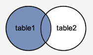
Fig 3: Left outer join

RIGHT OUTER JOIN

The RIGHT JOIN function is analogous to the LEFT JOIN function. This join retrieves all rows from the table on the right side of the join, as well as matching rows from the table on the left. The result-set will include null for the rows for which there is no matching row on the left side. RIGHT OUTER JOIN is another name for RIGHT JOIN.

Syntax

SELECT columns

FROM table1

RIGHT [OUTER] JOIN table2

ON table1.column = table2.column;

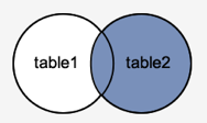
Fig 4: Right outer join

FULL OUTER JOIN

The result-set of FULL JOIN is created by combining the results of both LEFT JOIN and RIGHT JOIN. All of the rows from both tables will be included in the result-set. The result-set will contain NULL values for the rows for which there is no match.

Syntax

SELECT columns

FROM table1

FULL [OUTER] JOIN table2

ON table1.column = table2.column;

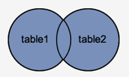
Fig 5: Full outer join

Q16) Explain the view?

A16) View

In SQL, a view is a virtual table based on the SQL statement result-set.

A view, much like a real table, includes rows and columns. Fields in a database view are fields from one or more individual database tables.

You can add SQL, WHERE, and JOIN statements to a view and show the details as if the data came from a single table.

Create a view

Syntax

CREATE VIEW view_name AS

SELECT column1, column2, ...

FROM table_name

WHERE condition;

Up-to-date data still displays a view! Any time a user queries a view, the database engine recreates the data, using the view's SQL statement.

Create a view example

A view showing all customers from India is provided by the following SQL.

CREATE VIEW [India Customers] AS

SELECT CustomerName, ContactName

FROM Customers

WHERE Country = 'India';

Updating a view

With the Build OR REPLACE VIEW command, the view can be changed.

Create or replace view syntax

CREATE OR REPLACE VIEW view_name AS

SELECT column1, column2, ...

FROM table_name

WHERE condition;

For the "City" view, the following SQL adds the "India Customers" column:

CREATE OR REPLACE VIEW [India Customers] AS

SELECT CustomerName, ContactName, City

FROM Customers

WHERE Country = 'India';

Dropping a view

With the DROP VIEW instruction, a view is removed.

Drop view syntax

DROP VIEW view_name;

"The following SQL drops the view of "India Customers":

DROP VIEW [India Customers];

Q17) Describe indexes?

A17) Indexes

Indexing is a technique for data structure that helps you to access information from a database file quickly. An Index is a small table of two columns only. The first column consists of a copy of a table's primary or candidate key. The second column includes a series of pointers to hold the disc block address where that particular key value is located.

Indexing is a way of maximizing a database's output by minimizing the amount of disc access needed when processing a question. It is a technique for data structure that is used to find and access the data in a database easily.

Using a few database columns, indexes are established.

• The first column is the Search key, which includes a copy of the table's primary or candidate key. In order for the corresponding data to be accessed easily, these values are stored in sorted order.
• The second column is the Data Reference or Pointer, which includes a series of pointers that hold the disc block address where you can find the particular key value.

Indexing has different attributes:

• Access Types: This refers to the access type, such as value-based quest, access to the range, etc.
• Access Time: This refers to the time taken to locate a single element of data or a collection of elements.
• Insertion Time: It relates to the time it takes to find a suitable space and insert new data.
• Deletion Time: It takes time to find and delete an object and to update the layout of the index.
• Space Overhead: It refers to the extra space that the index takes.

Q18) What are the types of indexes?

A18) Types of indexes

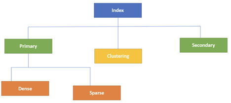
Fig 6: Types of database

1. Primary index

The Primary Index is an ordered file with two fields and a fixed length scale. The first field is the same as the primary key, and the second field is pointed to that particular block of information. In the primary index, the relationship between the entries in the index table is always one-to-one.

Main DBMS indexing is also further split into two forms:

• Dense
• Sparse

Dense index

In a dense index, for each search key valued in the database, a record is generated. This helps you to search more easily, however more space is required to store index records. Method records include the value of the search key in this index and point to the actual record on the disc.

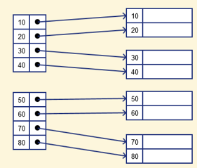
Fig 7: Dense index

Sparse index

It is an index record that only exists in the file for some of the values. The Sparse Index helps you solve the problems of DBMS Dense Indexing. A number of index columns store the same data block address in this form of indexing technique, and the block address will be fetched when data needs to be retrieved.

However, for only those search-key values, sparse Index stores index records. It requires less space, less overhead maintenance for insertion, and deletions, but compared to the dense index for locating records, it is slower.

The database index below is an example of the Sparse Index

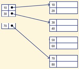
Fig 8: Sparse index

2.     Clustering index

The records themselves are stored in the index in a clustered index, and not the pointers. On non-primary key columns, the Index is often generated, which may not be unique for each record.

You can group two or more columns in such a situation to get unique values and create an index called the Clustered Index. This helps you locate the record faster as well.

Example:

Suppose a business has many staff in each department. Suppose we use a clustering index, where all employees within a single cluster who belong to the same Dept ID are considered, and index pointers point to the entire cluster. Dept Id is a non-unique key here.

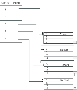
Fig 9: Example of cluster index

3.     Secondary index

In DBMS, a secondary index can be created by a field that has a specific value for each record and should be a candidate key. It is also known as an index for non-clustering.

To reduce the mapping size of the first level, this two-level database indexing technique is used. A wide range of numbers is chosen for the first level because of this; the mapping size still remains small.

In secondary indexing, another degree of indexing is added to reduce the mapping scale. The huge range for the columns is initially chosen in this process, so that the mapping scale of the first level becomes small. Each range is then further split into smaller ranges.

The first level mapping is stored in the primary memory, so that the fetching of addresses is easier. In the secondary memory, the second level mapping and actual data are stored (hard disk).

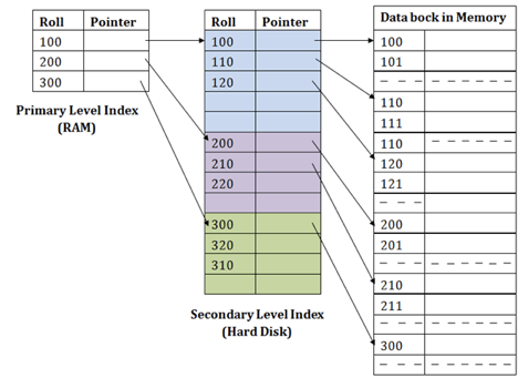
Fig 10: Secondary index

Let’s understand this by an example:

• If you want to find the record of roll 111 in the diagram, the first level index will look for the highest entry that is smaller than or equal to 111. At this amount, he'll get 100.
• Then again, it does max (111) <= 111 at the second index stage and gets 110. It now goes to the data block using the address 110, and starts looking for each record until it gets 111.
• This is how this approach is used to conduct a search. Often, adding, modifying or removing is performed the same way.

Q19) What is the difference between IN and BETWEEN operators?

A19) Difference between In and BETWEEN operators

Q20) Write the Difference between INNER JOIN and OUTER JOIN?

A20) Difference between INNER JOIN and OUTER JOIN