Unit-3

Database Design

Q1) What is a Good Database Design and what are their importance?

A1)

A good database design process is governed by specific rules. The first rule dictates that redundant data must be avoided; as it wastes space and increases the probability of faults and discrepancies within the database. The next rule is that the accuracy and comprehensiveness of information is extremely imperative. If the database contains erroneous information, any documents that fetch data from such a database will also include inaccurate information. Consequently, any decisions based on those documents will be misleading.

So, how can you ensure that your database design is good? A well-designed database is the one that:

ETL Your Enterprise Data Using MYSQL Connector

Move MySQL Data to a Destination of Your Choice Through a Codeless, Drag-and-Drop UI.

Importance of Database Design

Database design defines the database structure used for planning, storing, and managing information. Accuracy in data can only be accomplished if a database is designed to store only valuable and necessary information.

A well-designed database is imperative in guaranteeing information consistency, eliminating redundant data, efficiently executing queries, and improving the performance of the database. Meticulously designing a database saves you from wasting time and getting frustrated during the database development phase. A good database design also allows you to easily access and retrieve data whenever needed.

The reliability of data depends on the table structure; whereas creating primary and unique keys guarantees uniformity in the stored information. Data replication can be avoided by forming a table of probable values and using a key to denote the value. So, whenever the value changes, the alteration happens only once in the main table.

As the general performance of a database depends on its design, a good database design uses simple queries and faster implementation. It is easy to maintain and update; whereas fixing trivial interruptions in a poor database design may harm stored events, views, and utilities.

Q2) What is the database development life cycle?

A2)

Database Development Life Cycle

There are various stages in database development. However, it is not necessary to follow each of the steps sequentially. The life cycle can be broadly divided into three steps: requirement analysis, database designing, and implementation.

1- Requirement Analysis

Requirement analysis requires two steps:

2- Database designing

The actual database designing takes into account two key models:

3- Implementation

The implementation stage of database development life cycle is concerned with:

Q3) What is functional dependency?

A3)

Functional Dependency

Functional dependency (FD) is a set of constraints between two attributes in a relation. Functional dependency says that if two tuples have same values for attributes A1, A2,..., An, then those two tuples must have to have same values for attributes B1, B2, ..., Bn.

Functional dependency is represented by an arrow sign (→) that is, X→Y, where X functionally determines Y. The left-hand side attributes determine the values of attributes on the right-hand side.

Armstrong's Axioms

If F is a set of functional dependencies then the closure of F, denoted as F+, is the set of all functional dependencies logically implied by F. Armstrong's Axioms are a set of rules, that when applied repeatedly, generates a closure of functional dependencies.

Trivial Functional Dependency

Q4) Explain normalization in database and what are the different types of normalization

A4)

Normalization

If a database design is not perfect, it may contain anomalies, which are like a bad dream for any database administrator. Managing a database with anomalies is next to impossible.

Normalization is a method to remove all these anomalies and bring the database to a consistent state.

First Normal Form

First Normal Form is defined in the definition of relations (tables) itself. This rule defines that all the attributes in a relation must have atomic domains. The values in an atomic domain are indivisible units.

Fig 3 – 1NF

We re-arrange the relation (table) as below, to convert it to First Normal Form.

Fig 4 - Re-arrange the relation 1NF

Each attribute must contain only a single value from its pre-defined domain.

Second Normal Form

Before we learn about the second normal form, we need to understand the following −

If we follow second normal form, then every non-prime attribute should be fully functionally dependent on prime key attribute. That is, if X →A holds, then there should not be any proper subset Y of X, for which Y → A also holds true.

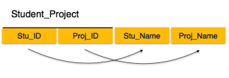
Fig 5 – 2 NF

We see here in Student_Project relation that the prime key attributes are Stu_ID and Proj_ID. According to the rule, non-key attributes, i.e. Stu_Name and Proj_Name must be dependent upon both and not on any of the prime key attribute individually. But we find that Stu_Name can be identified by Stu_ID and Proj_Name can be identified by Proj_ID independently. This is called partial dependency, which is not allowed in Second Normal Form.

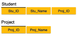
Fig 6 - Partial dependency

We broke the relation in two as depicted in the above picture. So there exists no partial dependency.

Third Normal Form

For a relation to be in Third Normal Form, it must be in Second Normal form and the following must satisfy −

Fig 7 – 3 NF

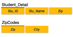
We find that in the above Student_detail relation, Stu_ID is the key and only prime key attribute. We find that City can be identified by Stu_ID as well as Zip itself. Neither Zip is a superkey nor is City a prime attribute. Additionally, Stu_ID→ Zip → City, so there existstransitive dependency.

To bring this relation into third normal form, we break the relation into two relations as follows −

Boyce-Codd Normal Form

Boyce-Codd Normal Form (BCNF) is an extension of Third Normal Form on strict terms. BCNF states that −

In the above image, Stu_ID is the super-key in the relation Student_Detail and Zip is the super-key in the relation ZipCodes. So,

Stu_ID→Stu_Name, Zip

and

Zip → City

Which confirms that both the relations are in BCNF.

Q5) What are the rules and types of functional dependency?

A5)

Rules of Functional Dependencies

Below are the Three most important rules for Functional Dependency in Database:

Types of Functional Dependencies in DBMS

There are mainly four types of Functional Dependency in DBMS. Following are the types of Functional Dependencies in DBMS:

Multivalued Dependency in DBMS

Multivalued dependency occurs in the situation where there are multiple independent multivalued attributes in a single table. A multivalued dependency is a complete constraint between two sets of attributes in a relation. It requires that certain tuples be present in a relation. Consider the following Multivalued Dependency Example to understand.

Example:

In this example, maf_year and color are independent of each other but dependent on car_model. In this example, these two columns are said to be multivalue dependent on car_model.

This dependence can be represented like this:

car_model ->maf_year

car_model-> colour

Trivial Functional Dependency in DBMS

The Trivial dependency is a set of attributes which are called a trivial if the set of attributes are included in that attribute.

So, X -> Y is a trivial functional dependency if Y is a subset of X. Let's understand with a Trivial Functional Dependency Example.

For example:

Consider this table of with two columns Emp_id and Emp_name.

{Emp_id, Emp_name} ->Emp_id is a trivial functional dependency as Emp_id is a subset of {Emp_id,Emp_name}.

Non Trivial Functional Dependency in DBMS

Functional dependency which also known as a nontrivial dependency occurs when A->B holds true where B is not a subset of A. In a relationship, if attribute B is not a subset of attribute A, then it is considered as a non-trivial dependency.

Example:

(Company} -> {CEO} (if we know the Company, we knows the CEO name)

But CEO is not a subset of Company, and hence it's non-trivial functional dependency.

Transitive Dependency in DBMS

A Transitive Dependency is a type of functional dependency which happens when t is indirectly formed by two functional dependencies. Let's understand with the following Transitive Dependency Example.

Example:

{Company} -> {CEO} (if we know the compay, we know its CEO's name)

{CEO } -> {Age} If we know the CEO, we know the Age

Therefore according to the rule of rule of transitive dependency:

{ Company} -> {Age} should hold, that makes sense because if we know the company name, we can know his age.

Note: You need to remember that transitive dependency can only occur in a relation of three or more attributes.

Closure of an Attribute: Closure of an Attribute can be defined as a set of attributes that can be functionally determined from it.

OR

Closure of a set F of FDs is the set F+ of all FDs that can be inferred from F

Closure of a set of attributes X concerning F is the set X+ of all attributes that are functionally determined by X

Pseudocode to find Closure of an Attribute?

Determine X+, the closure of X under functional dependency set F

X Closure : = will contain X itself;

Repeat the process as:

old X Closure     : = X Closure;

for each functional dependency P → Q in FD set do

if X Closure is subset of P then X Closure := X Closure U Q ;

Repeat until ( X Closure = old X Closure);

Algorithm of Determining X+, the Closure of X under F

Input: A set F of FDs on a relation schema R, and a set of attributes X, which is a subset of R.

 until (X+ = oldX+ ); 

7. QUESTIONS ON CLOSURE SET OF ATTRIBUTE:

1) Given relational schema R( P Q R S T U V) having following attribute P Q R S T U and V, also there is a set of functional dependency denoted by FD = { P->Q, QR->ST, PTV->V }.

Determine Closure of (QR)+ and (PR)+

a) QR+ = QR (as the closure of an attribute or set of attributes contain same).

Now as per algorithm look into a set of FD that complete the left side of any FD contains either Q, R, or QR since in FD QR→ST has complete QR.

Hence QR+ = QRST

Again, trace the remaining two FD that any left part of FD contains any Q, R, S, T.

Since no complete left side of the remaining two FD{P->Q, PTV->V} contain Q, R, S, T.

Therefore QR+ = QRST (Answer)

Note: In FD PTV→V, T is in QRST but that cannot be entertained, as complete PTV should be a subset of QRST

b) PR + = PR (as the closure of an attribute or set of attributes contain same)

Now as per algorithm look into a set of FD, and check that complete left side of any FD contains either P, R, or PR. Since in FD P→Q, P is a subset of PR, Hence PR+ = PRQ

Again, trace the remaining two FD that any left part of FD contains any P, R, Q, Since, in FD QR → ST has its complete left part QR in PQR

Hence PR+ = PRQST

Again trace the remaining one FD { PTV->V } that its complete left belongs to PRQST. Since complete PTV is not in PRQST, hence we ignore it.

Therefore PR+ = PRQST ( Answer)

2. Given relational schema R( P Q R S T) having following attributes P Q R S and T, also there is a set of functional dependency denoted by FD = { P->QR, RS->T, Q->S, T-> P }.

Determine Closure of ( T )+

T + = T (as the closure of an attribute or set of attributes contain same) Now as per algorithm look into a set of FD that complete the left side of any FD contains T since, in FD T → P, T is in T, Hence T+ = TP Again trace the remaining three FD that any left part of FD contain any TP, Since in FD P → QR has its complete left part P in TP, Hence T+ = TPQR Again trace the remaining two FD { RS->T, Q->S } that any of its Complete left belongs to TPQR, Since in FD Q → S has its complete left part Q in TPQR, Hence T+ = TPQRS Again trace the remaining one FD { RS->T } that its complete left belongs to TPQRS, Since in FD RS → T has its complete left part RS in TPQRS Hence T+ = TPQRS ( no changes, as T, is already in TPQRS) Therefore T+ = TPQRS ( Answer).

Q6) Explain normalization and what are its different types explain with examples

A6)

Normalization

Types of Normal Forms

There are the four types of normal forms:

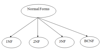
Fig 8 – Normal Forms

First Normal Form (1NF)

Example: Relation EMPLOYEE is not in 1NF because of multi-valued attribute EMP_PHONE.

EMPLOYEE table:

The decomposition of the EMPLOYEE table into 1NF has been shown below:

Second Normal Form (2NF)

Example: Let's assume, a school can store the data of teachers and the subjects they teach. In a school, a teacher can teach more than one subject.

TEACHER table

In the given table, non-prime attribute TEACHER_AGE is dependent on TEACHER_ID which is a proper subset of a candidate key. That's why it violates the rule for 2NF.

To convert the given table into 2NF, we decompose it into two tables:

TEACHER_DETAIL table:

TEACHER_SUBJECT table:

Third Normal Form (3NF)

A relation is in third normal form if it holds atleast one of the following conditions for every non-trivial function dependency X → Y.

Example:

EMPLOYEE_DETAIL table:

Super key in the table above:

Candidate key: {EMP_ID}

Non-prime attributes: In the given table, all attributes except EMP_ID are non-prime.

Here, EMP_STATE & EMP_CITY dependent on EMP_ZIP and EMP_ZIP dependent on EMP_ID. The non-prime attributes (EMP_STATE, EMP_CITY) transitively dependent on super key(EMP_ID). It violates the rule of third normal form.

That's why we need to move the EMP_CITY and EMP_STATE to the new <EMPLOYEE_ZIP> table, with EMP_ZIP as a Primary key.

EMPLOYEE table:

EMPLOYEE_ZIP table:

Boyce Codd normal form (BCNF)

Example: Let's assume there is a company where employees work in more than one department.

EMPLOYEE table:

In the above table Functional dependencies are as follows:

Candidate key: {EMP-ID, EMP-DEPT}

The table is not in BCNF because neither EMP_DEPT nor EMP_ID alone are keys.

To convert the given table into BCNF, we decompose it into three tables:

EMP_COUNTRY table:

EMP_DEPT table:

EMP_DEPT_MAPPING table:

Functional dependencies:

Candidate keys:

For the first table: EMP_ID
For the second table: EMP_DEPT
For the third table: {EMP_ID, EMP_DEPT}

Now, this is in BCNF because left side part of both the functional dependencies is a key.

Fourth normal form (4NF)

Example

STUDENT

The given STUDENT table is in 3NF, but the COURSE and HOBBY are two independent entity. Hence, there is no relationship between COURSE and HOBBY.

In the STUDENT relation, a student with STU_ID, 21 contains two courses, Computer and Math and two hobbies, Dancing and Singing. So there is a Multi-valued dependency on STU_ID, which leads to unnecessary repetition of data.

So to make the above table into 4NF, we can decompose it into two tables:

STUDENT_COURSE

STUDENT_HOBBY

Fifth normal form (5NF)

Example

In the above table, John takes both Computer and Math class for Semester 1 but he doesn't take Math class for Semester 2. In this case, combination of all these fields required to identify a valid data.

Suppose we add a new Semester as Semester 3 but do not know about the subject and who will be taking that subject so we leave Lecturer and Subject as NULL. But all three columns together acts as a primary key, so we can't leave other two columns blank.

So to make the above table into 5NF, we can decompose it into three relations P1, P2 & P3:

P1

P2

P3

Q7) Explain relational decomposition and what are its types

A7)

Relational Decomposition

Types of Decomposition

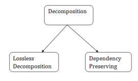
Fig 9 - Decomposition

Lossless Decomposition

Example:

EMPLOYEE_DEPARTMENT table:

The above relation is decomposed into two relations EMPLOYEE and DEPARTMENT

EMPLOYEE table:

DEPARTMENT table

Now, when these two relations are joined on the common column "EMP_ID", then the resultant relation will look like:

Employee ⋈ Department

Hence, the decomposition is Lossless join decomposition.

Dependency Preserving

Q8) What is multivalued dependency give an example?

A8)

Multivalued Dependency

Example: Suppose there is a bike manufacturer company which produces two colors(white and black) of each model every year.

Here columns COLOR and MANUF_YEAR are dependent on BIKE_MODEL and independent of each other.

In this case, these two columns can be called as multivalued dependent on BIKE_MODEL. The representation of these dependencies is shown below:

This can be read as "BIKE_MODEL multidetermined MANUF_YEAR" and "BIKE_MODEL multidetermined COLOR".

Q9) Explain Fourth normal form (4NF)

A10)

Example

STUDENT

The given STUDENT table is in 3NF, but the COURSE and HOBBY are two independent entity. Hence, there is no relationship between COURSE and HOBBY.

In the STUDENT relation, a student with STU_ID, 21 contains two courses, Computer and Math and two hobbies, Dancing and Singing. So there is a Multi-valued dependency on STU_ID, which leads to unnecessary repetition of data.

So to make the above table into 4NF, we can decompose it into two tables:

STUDENT_COURSE

STUDENT_HOBBY

Q10) Explain join dependency

A10)

Join Dependency