undefined | unit 3 modelling in time domain

UNIT-3MODELLING IN TIME DOMAIN Q1) Obtatin the state space representation for the given electircal system

A1) The state model is given as

Fig 1 State ModelThe state model shows that there are two energy storing elements L, C. As we already know that Number of state variables is equal to the number of energy storing elements.Hence we have two state variables[x1(t) and x2(t)]. We have one output V0(taken across capacitor) and input u(t).The output equation is then given as

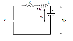
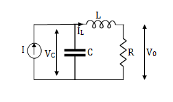
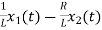
Y(t)=CX(t)+DU(t)

V0=Vc= x1(t) ….(a)

Hence output equation becomes

V0= x1(t)

y(t)=[1 0]+[0]u(t)

so, C=[1 0] D=[0]

Now writing the state equation

=Ax(t)+Bu(t)

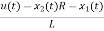
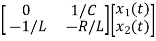
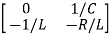
For that applying KVL in the above circuit

V=ILR+L+Vc

State Equation is =Ax(t)+Bu(t)

x1(t)=Vc

IL=C

=(1/C) x2(t) ……….(b)

VL=L

==VL/L

From KVL

L=VL=V-ILR-VC

= …………….(c)

From equation (b) and (c)

= [0 1/c]+ [0 0]u(t)

=[-1/L -R/L] + [1/L 0]

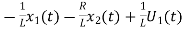
Now writing the state equation

=Ax(t)+Bu(t)

Hence A= B= A

Q2) Obtatin the state space representation for the given electircal system

A2) The state model shows that there are two energy storing elements L, C. As we already know that Number of state variables is equal to the number of energy storing elements.Hence we have two state variables[x1(t) and x2(t)]. We have one output V0(taken across capacitor) and input u(t).

Fig 2 State ModelHere output is V0. But from above electrical circuit V0=ILR

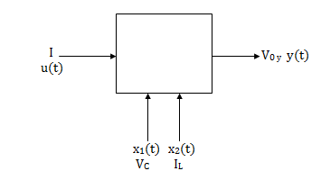
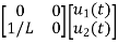
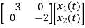
V0=x2(t)R

y(t)= V0= [0 R] + [0] u(t)

The output equation is given as

Y(t)=CX(t)+DU(t)

C=[0 R] D=[0]

Now finding state equation,we apply KCL in the given electrical circuit

I=IC+IL

But I-IL=IC

=x2(t)+ ……..(a)

=[0 1/C]+ [1/C 0] …….(b)

Applying KVL in the given electrical circuit we get

VC=VL+ILR

VC-ILR=VL=L

=[1/L -R/L] + [0] u(t) ………….(c)

From equation (b) and (c) we have

Now writing the state equation

=Ax(t)+Bu(t)

Hence A= B=

Note: We should always take voltage across the inductor L, and current through capacitor C. Q3) The closed loop transfer function is given as T(s)=

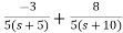
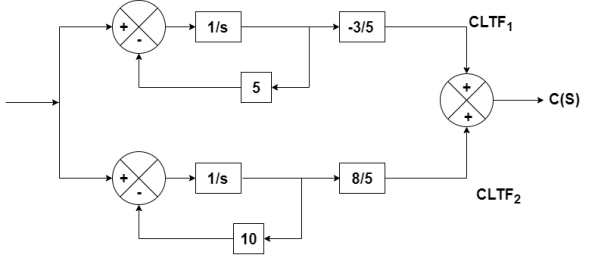
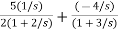
. Calculate the state model?A3) The transfer function can be simplified using partial fraction method as

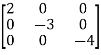
S+2=As+10A+Bs+5B

Equating coefficients of s from both sides

A+B=1

Equating coefficients of s0 from both sides

10A+5B=2

Solving above equations we get

A=-3/5

B=8/5

The transfer function will be

T(s)=

=-+

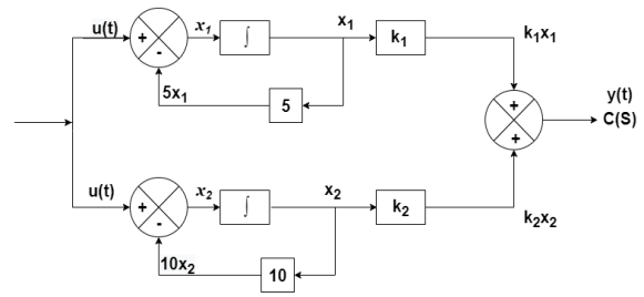
Number of poles= Number of energy storing elements

Fig 3 Block Diagram for T(s)=

The output equation is given as

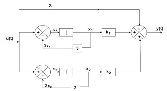
y(t)=k1x1(t)+k2x2(t)

y(t)= [k1 k2] + [0] [u(t)]

y(t)= [-3/5 8/5] + [0] [u(t)]

C=[-3/5 8/5]

D=0

From the above block diagram

=u(t)-5 x1

=-5x1+u(t)

=-10x2+u

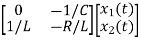
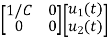
Therefore, the state equation is given as

Q4) The closed loop transfer function is given as T(s)=

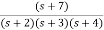
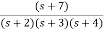
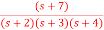. Calculate the state model?A4) The transfer function can be simplified using partial fraction method as

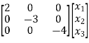
s+7=A[s2+7s+12] +B[s2+6s+8] +C[s2+5s+6]

Equating coefficients of s2 from both sides

A+B+C=0

Equating coefficients of s from both sides

7A+6B+5C=1

Equating coefficients of s0 from both sides

12A+8B+6C=7

Solving above equations and finding values of A, B and C

A=5/2

B=-4

C=3/2

The transfer function will be

T(s)=+

Fig 4 Block Diagram for T(s)=

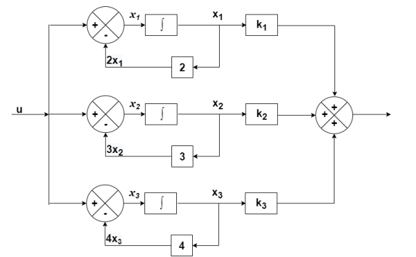
The output equation will be

y=k1x1+k2x2+k3x3

y=[k1 k2 k3][5/2 -4 3/2]

C=[5/2 -4 3/2]

D=[0]

The state equation is given as

=u(t)-2x1

=-2x1+u(t)

=-3x2+u

= -4x3+u

Therefore

= + [u]

Q5) The closed loop transfer function is T(s)=

. Find the state equation?A5) Here the number of poles = number of zeros

T(s)=

=2+

Solving above by partial fraction method

88= As+2A+Bs+3B

A=-B

2A+3B=88

A=-88

B=88

The transfer function becomes

T(s)= 2-

Fig 5 Block Diagram for T(s)=

The output equation will be

y(t)=2U+k1x1+k2x2

y=[-88 88]+[2]u

The output equation will be

=u(t)-3 x1

=-3x1+u(t)

=-2x2+u(t)

Therefore, the state equation is given as

Q6) The CLTF T(s)=

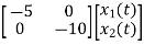
. Find the state equation?A6)

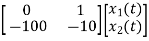
T(s)=

P1=2/s

P2=-8/s2

L1=-10/s

L2=-100/s2

Fig 6 SFG for T(s)=

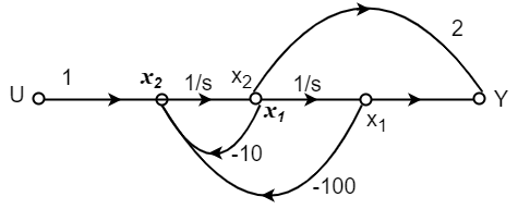
The state equation will be

=x2

=-10x2-100x1+u

Q7) Find the state equation from the given differential equation

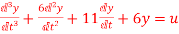A7) Let y=x1

==x2

==x3

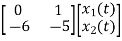
The above differential equation than becomes

+6+11 x2+6 x1=u

(t) =u-6(t)-11 x2-6 x1

Hence the state equation will be

= + [u]

Q8) For the given data below compute the transfer function of the systemA=

C=[1 0] and D=[0]A8) The state equation will be

=x1

=-6x1-5x2

From Equation (14)

= C{[SI-A]-1B} + D

=C{-}-1B+D

=C B+D

=[1 0] + 0

=+0

Q9) How can be obtain transfer function from the state space model?A9)

Fig 7 State modelThe above figure shows the state model of a system with two inputs u1(t) and u2(t), and having outputs y1(t) and y2(t). We know that the output equation is given as

Y(t)=Cx(t)+Du(t) (1)

(2)

Taking L.T of equation (1)

Y(s)=CX(s)+DU(s) (3)

Taking L.T of equation (2)

SX(s)=AX(s)+BU(s) (4)

X(s)=[SI-A]-1BU(s) (5)

Y(s)=CX(s)+DU(s)

Y(s)=C{[SI-A]-1BU(s)} + DU(s)

= C{[SI-A]-1B} + D (6)

[SI-A]-1=

The denominator of equation (6) is the characteristic equation

[SI-A]=0

Q10) What are the advantages of state space representation?A10) Few advantages are listed below:

The state space can be used for linear or nonlinear, time-variant or time-invariant systems.

It is easier to apply where Laplace transform cannot be applied.

The nth order differential equation can be expressed as 'n' equation of first order.

It is a time domain method.

As this is time domain method, therefore this method is suitable for digital computer computation.

On the basis of the given performance index, this system can be designed for an optimal condition.

Sign Up