undefined | unit 5 frequency domain techniques

Back to Study material

UNIT-5FREQUENCY DOMAIN TECHNIQUES Q1) sketch the bode plot for transfer function G(S) =

A1)

Replace S = j

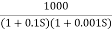
G(j=

This is type 0 system . so initial slope is 0 dB decade. The starting point is given as

20 log10 K = 20 log10 1000

= 60 dB

Corner frequency 1 = = 10 rad/sec

2 = = 1000 rad/sec

Slope after 1 will be -20 dB/decadetill second corner frequency i.e 2 after 2 the slope will be -40 dB/decade (-20+(-20)) as there are poles

2. For phase plot

= tan-1 0.1 - tan-1 0.001

For phase plot

100 -900

200 -9.450

300 -104.80

400 -110.360

500 -115.420

600 -120.00

700 -124.170

800 -127.940

900 -131.350

1000 -134.420

The plot is shown in figure 1

Fig 1 Magnitude Plot for G(S) =

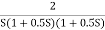
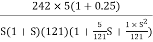
Q2) For the given transfer function determine G(S) =

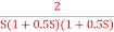Gain cross over frequency phase cross over frequency phase mergence and gain marginA2)

Initial slope = 1

N = 1 , (K)1/N = 2

K = 2

Corner frequency

1 = = 2 (slope -20 dB/decade

2 = = 20 (slope -40 dB/decade

2. phase

= tan-1 - tan-1 0.5 - tan-1 0.05

= 900- tan-1 0.5 - tan-1 0.05

1 -119.430

5 -172.230

10 -195.250

15 -209.270

20 -219.30

25 -226.760

30 -232.490

35 -236.980

40 -240.570

45 -243.490

50 -245.910

Finding gc (gain cross over frequency

M =

4 = 2 ( (

6 (6.25104) + 0.2524 +2 = 4

Let 2 = x

X3 (6.25104) + 0.2522 + x = 4

X1 = 2.46

X2 = -399.9

X3 = -6.50

For x1 = 2.46

gc = 3.99 rad/sec(from plot )

for phase margin

PM = 1800 -

= 900 – tan-1 (0.5×gc) – tan-1 (0.05 × gc)

= -164.50

PM = 1800 - 164.50

= 15.50

For phase cross over frequency (pc)

= 900 – tan-1 (0.5 ) – tan-1 (0.05 )

-1800 = -900 – tan-1 (0.5 pc) – tan-1 (0.05 pc)

-900 – tan-1 (0.5 pc) – tan-1 (0.05 pc)

Taking than on both sides

Tan 900 = tan-1

Let tan-1 0.5 pc = A, tan-1 0.05 pc = B

= 00

= 0

1 =0.5 pc 0.05pc

pc = 6.32 rad/sec

The plot is shown in figure 2.

Fig 2 Magnitude Plot G(S) =

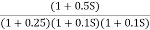
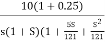
Q3)For the given transfer function G(S) =

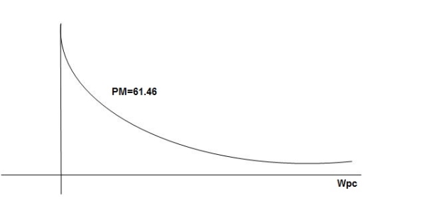
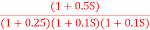Plot the rode plot find PM and GMA3)

T1 = 0.5 1 = = 2 rad/sec

Zero so, slope (20 dB/decade)

T2 = 0.2 2 = = 5 rad/sec

Pole , so slope (-20 dB/decade)

T3 = 0.1 = T4 = 0.1

3 = 4 = 10 (2 pole ) (-40 db/decade)

Initial slope 0 dB/decade till 1 = 2 rad/sec
From 1 to2 (i.e. 2 rad /sec to 5 rad/sec) slope will be 20 dB/decade
From 2 to 3 the slope will be 0 dB/decade (20 + (-20))
From 3 ,4 the slope will be -40 dB/decade (0-20-20)

Phase plot

= tan-1 0.5 - tan-1 0.2 - tan-1 0.1 - tan-1 0.1

500 -177.30

1000 -178.60

1500 -179.10

2000 -179.40

2500 -179.50

3000 -179.530

3500 -179.60

GM = 00

PM = 61.460

The plot is shown in figure 3

Fig 3 Magnitude and phase Plot for G(S) =

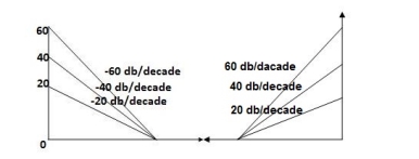
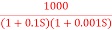
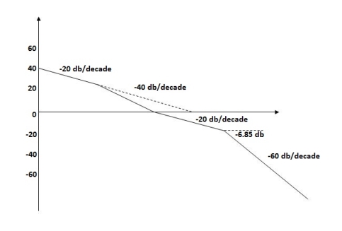
Q4) For the given transfer function plot the bode plot (magnitude plot) G(S) =

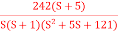A4) Given transfer function

G(S) =

Converting above transfer function to standard from

G(S) =

As type 1 system , so initial slope will be -20 dB/decade
Final slope will be -60 dB/decade as order of system decides the final slope
Corner frequency

T1 = , 11= 5 (zero)

T2 = 1 , 2 = 1 (pole)

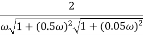
4. Initial slope will cut zero dB axis at

(K)1/N = 10

i.e = 10

5. finding n and

T(S) =

T(S)=

Comparing with standard second order system equation

S2+2ns +n2

n = 11 rad/sec

n = 5

11 = 5

= = 0.27

5. Maximum error

M = -20 log 2

= +6.5 dB

6. As K = 10, so whole plot will shift by 20 log 10 10 = 20 dBThe plot is shown in figure 4

1..JPG

Fig 4 Magnitude Plot for G(S) =

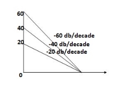
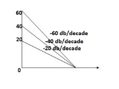
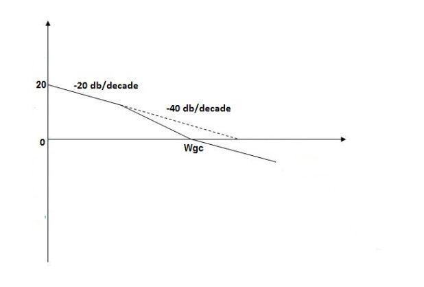
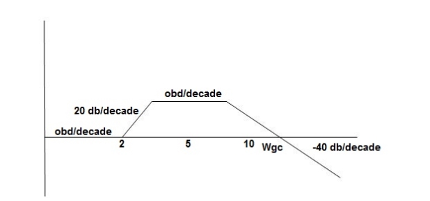
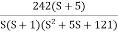Q5) For the given plot determine the transfer function

Fig 5 Magnitude PlotA5) From figure 5 we can conclude that

Initial slope = -20 dB/decade so type -1

Initial slope all 0 dB axis at

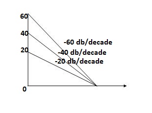
= 10 so

K1/N N = 1(K)1/N = 10.3. corner frequency

1 =

= 0.2 rad/sec

2 =

= 0.125 rad/sec3. At

= 5 the slope becomes -40 dB/decade, so there is a pole at

= 5 as slope changes from -20 dB/decade to -40 dB/decade4. At

= 8 the slope changes from -40 dB/decade to -20 dB/decade hence 5. is a zero at

= 8 (-40+(+20) = 20)Hence transfer function is T(S) =

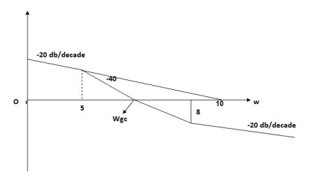
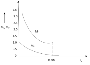
Q6) Explain correlation between time and frequency response?A6) The transfer function of second order system is shown as

C(S)/R(S) = W2n / S2 + 2ξWnS + W2n - - (1)

ξ = Ramping factor

Wn = Undamped natural frequency for frequency response let S = jw

C(jw) / R(jw) = W2n / (jw)2 + 2 ξWn(jw) + W2n

Let U = W/Wn above equation becomes

T(jw) = W2n / 1 – U2 + j2 ξU

so,

| T(jw) | = M = 1/√(1 – u2)2 + (2ξU)2 - - (2)

T(jw) = φ = -tan-1[ 2ξu/(1-u2)] - - (3)

For sinusoidal input the output response for the system is given by

C(t) = 1/√(1-u2)2 + (2ξu)2Sin[wt - tan-1 2ξu/1-u2] - - (4)

The frequency where M has the peak value is known as Resonant frequency Wn. This frequency is given as (from eqn (2)).

dM/du|u=ur = Wr = Wn√(1-2ξ2) - - (5)

from equation(2) the maximum value of magnitude is known as Resonant peak.

Mr = 1/2ξ√1-ξ2 - - (6)

The phase angle at resonant frequency is given as

Φr = - tan-1 [√1-2ξ2/ ξ] - - (7)

As we already know for step response of second order system the value of damped frequency and peak overshoot are given as

Wd = Wn√1-ξ2 - - (8)

Mp = e- πξ2|√1-ξ2 - - (9)

The comparison of Mr and Mp is shown in figure(1). The two performance indices are correlated as both are functions of the damping factor ξ only. When subjected to step input the system with given value of Mr of its frequency response will exhibit a corresponding value of Mp.

Fig 6 Frequency Domain SpecificationSimilarly the correlation of Wr and Wd is shown in fig(6) for the given input step response [ from eqn(5) & eqn(8) ]Wr/Wd = √(1- 2ξ2)/(1-ξ2)Mp = Peak overshoot of step responseMr = Resonant Peak of frequency responseWr = Resonant frequency of Frequency responseWd = Damping frequency of oscillation of step response.From fig above it is clear that for ξ> 1/2, value of Mr does not exists. Q7) For the transfer function below plot the Nyquist plot and also comment on stability G(S) = 1/S+1A7) N = Z – P (No pole of right half of S plane P = 0 )P = 0, N = Z

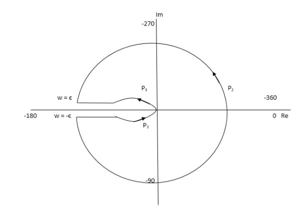
NYQUIST PATH :-

P1 = W – (0 to - ∞)

P2 = ϴ( - π/2 to 0 to π/2 )

P3 = W(+∞ to 0)

Fig 7 Nyquist path

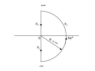
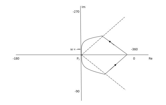
Substituting S = jw

G(jw) = 1/jw + 1

M = 1/√1+W2

Φ = -tan-1(W/I)

for P1 :- W(0 to -∞)

W M φ

0 1 0

-1 1/√2 +450

-∞ 0 +900

Path P2 :-

W = Rejϴ R  ∞ϴ -π/2 to 0 to π/2

G(jw) = 1/1+jw

= 1/1+j(Rejϴ) (neglecting 1 as R  ∞)

M = 1/Rejϴ = 1/R e-jϴ

M = 0 e-jϴ = 0

Path P3 :-

W = -∞ to 0

M = 1/√1+W2 , φ = -tan-1(W/I)

W M φ

∞ 0 -900

1 1/√2 -450

0 1 00

The Nyquist Plot is shown in fig below

Fig 8 Nyquist Plot G(S) = 1/S+1 From plot we can see that -1 is not encircled so, N = 0But N = Z, Z = 0So, system is stable.Q8) for the transfer function below plot the Nyquist Plot and comment on stability G(S) = 1/(S + 4)(S + 5)A8) N = Z – P , P = 0, No pole on right half of S-planeN = ZNYQUIST PATHP1 = W(0 to -∞)P2 = ϴ(-π/2 to 0 to +π/2)P3 = W(∞ to 0)

Fig 9 Nyquist Path

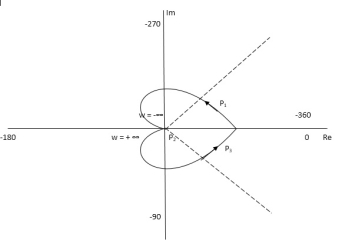
Path P1 W(0 to -∞)

M = 1/√42 + w2 √52 + w2

Φ = -tan-1(W/4) – tan-1(W/5)

W M Φ

0 1/20 00

-1 0.047 25.350

-∞ 0 +1800

Path P3 will be the mirror image across the real axis.

Path P2 :ϴ(-π/2 to 0 to +π/2)

S = Rejϴ

G(S) = 1/(Rejϴ + 4)( Rejϴ + 5)

R∞

= 1/ R2e2jϴ = 0.e-j2ϴ = 0

The plot is shown in fig below. From plot N=0, Z=0, system stable.

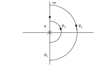
Fig 10 Nyquist Plot G(S) = 1/(S + 4)(S + 5)Q9) For the given transfer function, plot the Nyquist plot and comment on stability G(S) = k/S2(S + 10)?A9) As the poles exists at origin. So, first time we do not include poles in Nyquist plot. Then check the stability for second case we include the poles at origin in Nyquist path. Then again check the stability.PART – 1 : Not including poles at origin in the Nyquist Path.

Fig 11 Nyquist Path

P1 W(∞ Ɛ) where Ɛ 0

P2 S = Ɛejϴ ϴ(+π/2 to 0 to -π/2)

P3 W = -Ɛ to -∞

P4 S = Rejϴ, R  ∞, ϴ = -π/2 to 0 to +π/2

For P1

M = 1/w.w√102 + w2 = 1/w2√102 + w2

Φ = -1800 – tan-1(w/10)

W M Φ

∞ 0 -3 π/2

Ɛ ∞ -1800

Path P3 will be mirror image of P1 about Real axis.

G(Ɛ ejϴ) = 1/( Ɛ ejϴ)2(Ɛ ejϴ + 10)

Ɛ 0, ϴ = π/2 to 0 to -π/2

= 1/ Ɛ2 e2jϴ(Ɛ ejϴ + 10)

= ∞. e-j2ϴ [ -2ϴ = -π to 0 to +π ]

Path P2 will be formed by rotating through -π to 0 to +π

Path P4 S = Rejϴ R  ∞ ϴ = -π/2 to 0 to +π/2

G(Rejϴ) = 1/ (Rejϴ)2(10 + Rejϴ)

= 0

N = Z – P

No poles on right half of S plane so, P = 0

N = Z – 0

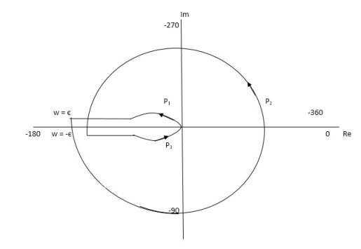
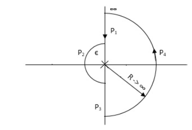
Fig 12 Nyquist Plot for G(S) = k/S2(S + 10)But from plot shown in fig 12. it is clear that number of encirclements in Anticlockwise direction. So,N = 2N = Z – P2 = Z – 0Z = 2Hence, system unstable.PART 2 Including poles at origin in the Nyquist Path.

Fig 13 Nyquist Path

P1 W(∞ to Ɛ) Ɛ 0

P2 S = Ɛejϴ Ɛ 0 ϴ(+π/2 to +π to +3π/2)

P3 W(-Ɛ to -∞) Ɛ 0

P4 S = Rejϴ, R  ∞, ϴ(3π/2 to 2π to +5π/2)

M = 1/W2√102 + W2 , φ = - π – tan-1(W/10)

P1 W(∞ to Ɛ)

W M φ

∞ 0 -3 π/2

Ɛ ∞ -1800

P3( mirror image of P1)

P2 S = Ɛejϴ

G(Ɛejϴ) = 1/ Ɛ2e2jϴ(10 + Ɛejϴ)

Ɛ 0

G(Ɛejϴ) = 1/ Ɛ2e2jϴ(10)

= ∞. e-j2ϴϴ(π/2 to π to 3π/2)

-2ϴ = (-π to -2π to -3π)

P4 = 0

Fig 14 Nyquist Plot G(S) = k/S2(S + 10)The plot is shown in fig above. from the plot it is clear that there is no encirclement of -1 in Nyquist path. (N = 0). But the two poles at origin lies to the right half of S-plane in Nyquist path.(P = 2)[see path P2]N = Z – P0 = Z – 2Z = 2Hence, system is unstable.Path P2 will be formed by rotating through -π to -2π to -3πQ10) Write the frequency domain specifications?A10) Resonant Peak (Mr): The maximum value of magnitude is known as Resonant peak. The relative stability of the system can be determined by Mr. The larger the value of Mr the undesirable is the transient response.Resonant Frequency (Wr): The frequency at which magnitude has maximum value.Bandwidth: The band of frequencies lying between -3db points.Cut-off frequency –The frequency at which the magnitude is 3db below its zero frequency.Cut-off Rate – It is the slope of the log magnitude curve near the cut off frequency.

Sign Up