Transportation Models Introduction
Question Bank
Q1) Define Assignment model.
A1) Given n promotion and n jobs, it's clear that there are n allocations during this case. Each facility or worker can perform each job, one at a time. However, certain steps are required to form the allocation so as to maximize profits or minimize costs or time.
In this table, Coij is defined because the cost when the jth job is assigned to the ith worker. Note that this is often a special case of transportation problems when the number of rows is adequate to the amount of columns.
Mathematical formulation:
The basic viable solution to the allocation problem consists of (2n – 1) variables, where the (n – 1) variable is zero and n is that the number of jobs or facilities. thanks to this high degree of degeneracy, solving problems with normal shipping methods are often a posh and time-consuming task. Therefore, another method springs. it's vital to formulate the matter before proceeding to absolutely the law.
Suppose xjj may be a variable defined as follows:
If the primary job is assigned to the jth machine or facility
0 if the i-th job isn't assigned to the j-th machine or facility.
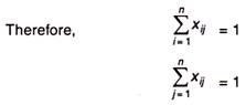
Here, the matter is made one-to-one, or one job is assigned to at least one facility or machine.
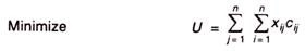
The total allocation cost is
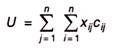
The above definition is often evolved into a mathematical model as follows:
Determine xij> 0 (i, j = 1,2,3… n),
Be constrained
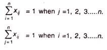
xij is either 0 or 1.
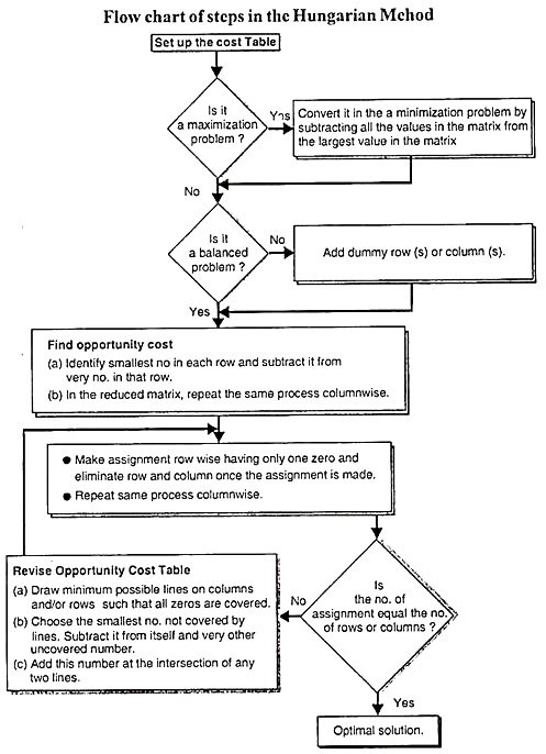
Q2) How to solve the matter by Hungarian technique?
A2) Consider a minimization type objective function. Resolving this allocation issue involves the subsequent steps:
1. Find the littlest cost element in each row of the required cost table, starting with the primary row. Here, this smallest element is subtracted from each element therein row. Therefore, get a minimum of one zero in each row of this new table.
2. After creating the table (as in step 1), get the columns of the table. Start with the primary column and find rock bottom cost think about each column. Then subtract this smallest element from each element therein column. After performing steps 1 and a couple of, you'll see a minimum of one zero in each column of the reduced cost table.
3. The reduced table is now allocated within the following way:
(I) Rows are continuously inspected until a row with just one zero is found. This assignment to one zero is formed by placing a square □ around it, with all other zeros being strikethrough (x) within the corresponding column. this is often because they're not used for other assignments during this column. The steps are performed for every row.
(II) Step 3 (i) am performed on the column as follows: -Columns are continuously inspected until a column with just one zero is found. Now, by placing a square around it, this single zero is assigned, and at an equivalent time all other zeros within the corresponding row are erased (x) A step is performed on each column. I will.
(III) Steps 3, (i), and three (ii) are repeated until all zeros are marked or strikethrough is drawn. Here, if the amount of zeros marked or the amount of allocations made is adequate to the amount of rows or columns, the simplest solution is achieved. There’s exactly one assignment for every column or column, with none assignment. During this case, attend step 4.
4. At this stage, draw the minimum number of lines (horizontal and vertical) needed to hide all the zeros within the matrix obtained in step 3. Use the subsequent procedure.
(i) Put a check on all unassigned lines.
(ii) Now mark of these columns that have zeros within the graduated rows (iii) Now check all rows that haven't yet been marked and are assigned to the marked columns.
(iv) All steps, namely (4 (i), 4 (ii), 4 (iii), are repeated until no row or column are often marked.
(V) Draw a line through all unmarked rows and marked columns. Also note that in an n x n matrix, lines but "n" always cover all zeros if there's no solution between them.
5. In step 4, the number of lines drawn is n orthe number of lines, it's the best solution. If not, go to step 6.
6. Select the smallest element from all uncovered elements. Here, this element is subtracted from all uncovered elements and added to the element at the intersection of the two lines. This is the new allocation matrix.
7. Repeat step (3) until the number of allocations is equal to the number of rows or columns.
Q3) Explain the Balanced and Unbalanced Problems.
A3) Whenever the cost matrix of an allocation problem is not a square matrix, that is, the number of sources is not equal to the number of destinations, the allocation problem is called an imbalanced allocation problem. In such problems, dummy rows (or columns) are added to the matrix to make a matrix. The dummy row or column contains all cost elements as zero. The Hungarian method could also be wont to solve the matter.
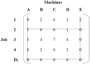
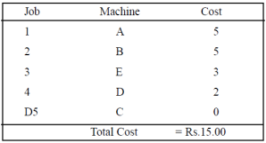
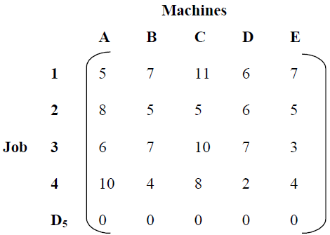
Example: A company has 5 machines used for 4 jobs. Each job can only be given to one machine. The following table shows the cost of each job on each machine.
Example of an unbalanced maximization allocation problem
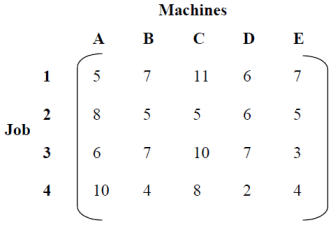
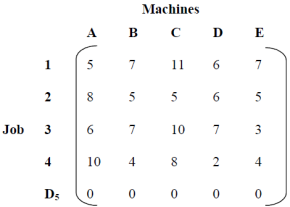
Solution: Add dummy row D5 to convert the 4x5 matrix to a square matrix.
Dummy line D5 has been added
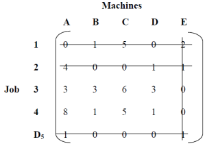
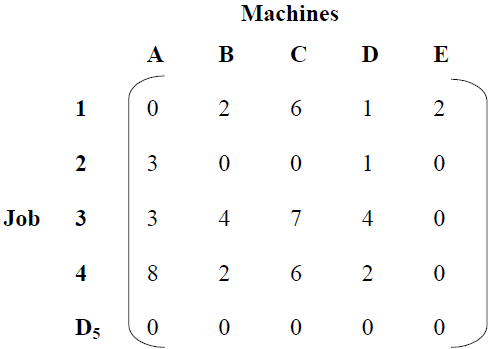
Matrix row direction reduction
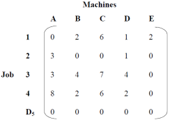
No per-column reduction is required as every column contains a single zero. Then draw the minimum number of lines that cover all zeros, as shown in the table.
All zeros in the matrix of interest
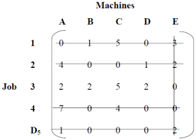
Number of lines drawn ≠ Matrix order. Therefore, it is not optimal.
As shown in the table, select the least covered element, that is, 1, subtract it from the other uncovered elements, add it to the element at the intersection of the lines, and cover it with a single line. Do not change the element.
Subtract or add to an element
Number of lines drawn ≠ Matrix order. Therefore, it is not optimal.
Add or subtract 1 again from the element
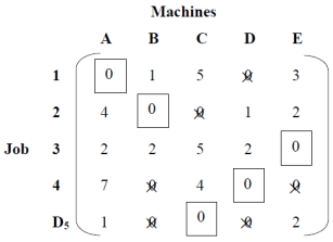
Number of lines drawn = degree of matrix. Therefore, optimality is reached. Then assign the job to the machine, as shown in the table.
Assigning jobs to machines
Example: In a plant layout, four different machines M1, M2, M3, and M4 are installed in a machine shop. There are five missing areas: A, B, C, D and E. Due to limited space, Machine M2 cannot be installed in Area C and Machine M4 cannot be installed in Area A. The installation cost of the machine is shown in the table.
Q4) What steps are used in Hungarian method?
A4) The Hungarian methods are often summarized within the following steps:
Step 1: Create a price table from the given problem.
If the number of rows isn't adequate to the number of columns, or the other way around, you would like to feature dummy rows or columns. The value of allocating dummy cells is usually zero.
Step 2: Find the chance Cost Table:
(A) Find the littlest element in each row of the required cost table and subtract it from each element therein row.
(B) Within the reduction matrix obtained from 2 (a), find the littlest element in each column and subtract it from each element. Each row and column has a minimum of one zero value.
Step 3: Make an allocation within the cost Matrix:
The allocation procedure is as follows:
(A) Examine the rows continuously until you get a row with just one unmarked zero. Make the assignment one zero by creating a square around it.
(B) For every zero-value assigned, delete (cancel) all other zeros within the same row and / or column.
(C) Repeat steps 3 (a) and three (b) for every column, leaving just one unassigned zero value.
(D) If there are two or more unmarked zeros within the rows and / or columns and therefore the check cannot select one, select any assigned zero cell.
(E) Continue this process until all zeros within the matrix are enclosed (assigned) or deleted (x).
Step 4: Optimal criteria:
If the assigned cell members are adequate to the row sequence that is the best solution. The entire cost related to this solution is obtained by adding the first cost figure to the occupied cell.
If zero cells are arbitrarily selected in step (3), an alternate optimal solution exists. However, if you can't find the simplest solution, attend step (5).
Step 5: Modify the chance cost table.
Use the subsequent procedure to draw a group of horizontal and vertical lines that cover all zeros within the revised cost table obtained in step (3).
(A) Add a check (√) to every row that has not been assigned.
(B) Examine the marked line. If zeros occur in these columns, check each row that contains the assigned zeros.
(C) Repeat this process until you'll not mark rows or columns.
(D) Draw a line through each marked column and every unmarked row.
If the number of drawn lines is adequate to the amount (or columns), then the present solution is that the best solution otherwise, attend step 6.
Step 6: Create a newly revised cost Table.
(A) Select the littlest element from the cells that aren't covered by the road, and call this value K.
(B) Draw K from all the weather within the cell that isn’t covered by the road.
(C) Add K to the element within the cell covered by the 2 lines, that is, the intersection of the 2 lines.
(D) The weather of the cell covered by one row aren't changed.
Step 7: Repeat steps 3-6 close up the lights for the simplest solution
Q5) Write note on balanced transportation issues.
A5) For shipping issues:
Minimize z =
Be constrained


If the aggregate supply from all sources is equal to the aggregate demand of all destinations, then x11 of all i and j is said to be a balanced transport problem, otherwise the problem is an imbalanced transport problem is said to be.
There may be a solution that can only be implemented if the transportation problem is a balanced problem. Imbalanced issues can be balanced by adding dummy supply centers (rows) or dummy demand centers, depending on your requirements.
Q6) Explain Prohibited Transportation Problems, Unique or Multiple Optimal Solutions.
A6) Sometimes, there may be situations when a particular route cannot be used for transportation, for example, when road is being constructed, accidents, floods, etc. These problems are known as prohibited transportation problems. These can be solved by two methods:
It is possible that a transportation problem to have multiple optimal solutions. This happens when one or more of the improvement indices are zero in the optimal solution. This means that there is a possibilityfor designing alternative shipping routes with the same total shipping cost. The alternate optimal solution can be found by shipping the most to this unused square using a stepping-stone path. In the real world, alternate optimal solutions help with better management and greater flexibility in selecting and using resources.
Consider the following transportation problem.
Factory | Warehouse | Supply | ||
W1 | W2 | W3 | ||
F1 | 16 | ∞ | 12 | 200 |
F2 | 14 | 8 | 18 | 160 |
F3 | 26 | ∞ | 16 | 90 |
Demand | 180 | 120 | 150 | 450 |
Solution:
As can be seen in the question, we have some restrictions.
An initial solution is obtained by the matrix minimum method
Final Table
Factory | Warehouse | Supply | ||
W1 | W2 | W3 | ||
F1 |
| ∞ |
| 200 |
F2 |
|
| 18 | 160 |
F3 |
| ∞ | 16 | 90 |
Demand | 180 | 120 | 150 | 450 |


16 X 50 + 12 X 150 + 14 X 40 + 8 X 120 + 26 X 90 = 6460.
The minimum transportation cost is Rs. 6460.
Q7) Elaborate and write Simple Formulation of Transportation Problems.
A7) While solving problem, the key part lies in formulating the model by decoding the problem. For a transportation problem, usually, the problem will be given in a tabular form or matrix form called transportation table or cost-effective matrix.
Let’s check an example below.
|
| DESTINATIONS |
|
| SUPPLY |
|
| 1 | 2 | 3 |
|
| A | 2 | 3 | 1 | 10 |
SOURCE | B | 5 | 4 | 8 | 35 |
| C | 5 | 6 | 8 | 25 |
DEMAND |
| 20 | 25 | 25 |
|
An example for transportation problem with Source{A,B,C} with total supply as 70 and Destinations{1,2,3} with total demand as 70.
Here,
Source = {A, B, C}
They represent sources with supply capacity 10,35,25 units of commodities respectively (given in orange)
Hence, total supply=10+35+25=70
Destinations= {1,2,3}
They represent destinations that require 20,25,25 units of commoditiesrespectively (given in green).Hence, total demand=20+25+25=70The elements represented in the matrixare called cost. i.e., the unit cost involved in moving unit commodity from one origin to another destination.
For example,
The cost incurred in moving 1 unit of the commodity from source A to destination 1= ₹2/-
The cost incurred in moving 1 unit of the commodity from source A to destination 1= ₹2/- (here, we are looking at the cross-section of source A and destination 1)
Likewise,
The cost incurred in moving one unit of the commodity from source B to destination 2= ₹4and so on. [Here, we are looking at the cross-section of source and destination].
Q8) How will you explain North West Corner Rule (NWCR).
A8) Northwest corner rule
Example
Start with an empty matrix with supply at the bottom and supply at the right.
When you get the cell in the northwest corner, its values are the minimum d1 and s1. Since s₁ is smaller than d₁, cancel the first line.
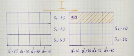
In the next iteration, do the same steps.
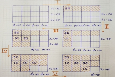
We come up with such a table and a basic viable solution.
Q9) Define Least Cost Method (LCM).
A9) There are several methods available to get the first basic viable solution to your shipping problem. Only the following three are discussed here. To find the first basic viable solution, the total supply should be equal to the total demand.
Method: Least common multiple method (LCM)
The lowest cost method is more economical than the northwest corner rule because it starts with a low starting cost. The various steps involved in this method are summarized below.
Step 1: Find the cell with the lowest (minimum) cost in the transport table.
Step 2: Assign the maximum amount that can be executed in this cell.
Step: 3: Delete the row or column to which the assignment will be made.
Step: 4: Repeat the above steps for the reduced transport table until all allocations are complete.
Example
Use the lowest cost method to get the first basic viable solution to the next shipping problem.
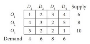
Here, Oi and Dj indicate the i-th starting point and the j-th destination, respectively.
Solution:
Total supply = total demand = 24
The problem given is a balanced transportation problem.
Therefore, there is a viable solution to the given problem.
Q10) How initial basic feasible solution is is obtained by VAM?
A10) The Vogel’s Approximation Method or VAM can be defined as an iterative procedure which is used to find out the initial feasible solution of the transportation problem. The initial basic feasible solution obtained by VAM is either optimal solution or very nearer to the optimal solution. Let’s go through the procedure with an example.
Example:
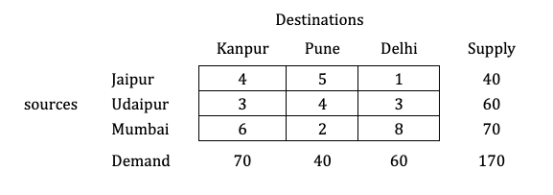
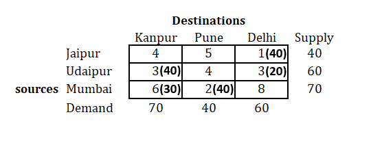
A mobile phone manufacturing company has three branches which are located in three different regions, say Jaipur, Udaipur and Mumbai. The company is supposed to transport mobile phones to three destinations, say Kanpur, Pune and Delhi. The availability from Jaipur, Udaipur and Mumbai is 40, 60 and 70 units respectively. The demand at Kanpur, Pune and Delhi are 70, 40 and 60 respectively. The transportation cost is shown in the matrix below (in Rs). Use the Vogel’s Approximation Method to find a basic feasible solution (BFS).

Solution:
Step 1: Balance the problem
Balance the problem meaning we need to check that if;
∑ Supply=∑ Demand
If this condition is satisfied, then we will consider the given problem as a balanced problem.
Now, what if it’s not balanced?
i.e., Σ Supply≠Σ Demand
If such a condition occurs, then we have to add a dummy source or market; whichever makes the problem balanced.
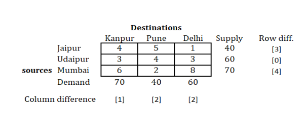
Step 2: Find out the Row difference and the Column difference
Now, we will find out the row and the column difference of the provided matrix.
For the same we will solve this as follows:

Here as you can see in the first row, we need to find out cell containing smallest value (least cost), and the second least.
Hence, we find 1 and 4 as the two lowest values in the first row.
Take the difference of these two numbers, i.e. (4−1)=3.
In a similar manner, find out differences for all the rows as shown above.
The same procedure is to be done with columns.
So, for the first column, you will get, (4−3)=1.
Find out difference for all columns as done above.
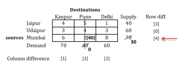
Step 3: Select the row/column with highest difference

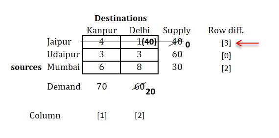
As we can see above, the highest difference value is 4 which is for the last row.
So we will select that row, and find out the minimum cost in that row.
You will find that, minimum cost is 2.
Now, compare the supply and demand for this row and column respectively.
We find that, we have supply as 70 and demand as 40 for the selected cell.
Compare both and select the minimum of them for the allocation in the cell, as shown below.
Cross out the column whose demand is fulfilled.
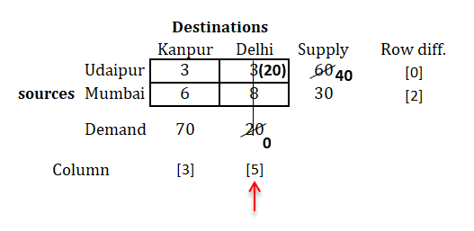
Step 4: Remove the row/column whose supply or demand is fulfilled and prepare new matrix and repeat the same procedure
As it can be seen, we now have a new matrix with second column removed (as its demand was 40 which was fulfilled)
Now, we will repeat the same procedure until we're done with all allocations.
i.e.,
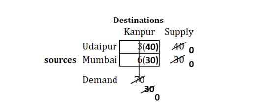
Step 5: After all the allocations are completed, write all the allocations in the matrix and find Transportation cost

We have all allocations with their respective cell now.
Find transportation cost as follows:
Transportation cost= (1x40)+(3x40)+(3x20)+(6x30)+(2x40)=Rs 480.
Q11) How do we find Optimal Solution by Modified Distribution (MODI) Method? (u, v and ∆)
A11) There are two steps to solving a transportation problem. The first phase requires finding the first basic viable solution, and the second phase optimizes the first basic viable solution obtained in the first phase. There are three ways to find the first basic viable solution.
This article describes how to optimize your first basic viable solution through the examples provided. Consider the following transportation problem.
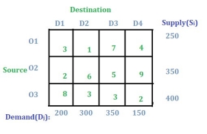
Solution:
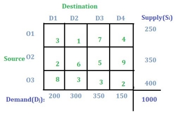
Step 1: Check if the problem is balanced.
If the sum of all supplies from sources O1, O2, and O3 is equal to the sum of all demands for destinations D1, D2, D3, and D4, then the shipping problem is a balanced shipping problem.
Note: If the problem is not imbalanced, you can follow the concept of dummy rows or columns to transform an imbalanced problem into equilibrium, as described in this article.
Step 2: Find the first basic viable solution.
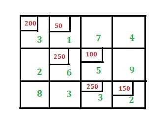
You can use one of the three methods described above to find the first basic viable solution. Here we use the Northwest Corner method. And according to the Northwest Corner Method, this is the final first basic viable solution.
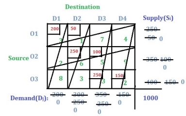
Now the total shipping cost is (200 * 3) + (50 * 1) + (250 * 6) + (100 * 5) + (250 * 3) + (150 * 2) = 3700.
Step 3: U-V method to optimize the first basic viable solution.
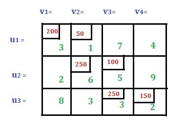
Below is the first basic viable solution.
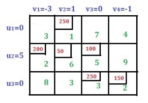
– For U-V methods, you need to find the row and column values ui and vj, respectively. Since we have 3 rows, we need to find 3 ui values. That is, u1 on the first row, u2 on the second row, and u3 on the third row.
Similarly, for four columns, you need to find the four vj values, v1, v2, v3, and v4. Please check the image below.
There is another formula for finding ui and vj.
ui + vj = Cij where Cij is the cost value of the assigned cell only. Please check this out for details.
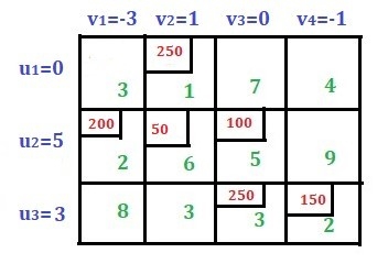
Before applying the above formula, we need to make sure that m + n – 1 is equal to the total number of cells allocated. Where m is the total number of rows and n is the total number of columns.
In this case, m = 3, n = 4, and the total number of cells allocated is 6, so m + n – 1 = 6. Later post if m + n – 1 is not equal to the total number of allocated cells.
Now assign any of the three u or any of the four v as 0 to find the values for u and v. In this case, assign u1 = 0. Then, using the above formula, we get v1 = 3 as u1 + v1 = 3 (that is, C11) and v2 = 1 as u1 + v2 = 1 (that is, C12). Similarly, we got the value of v2 = 1, so we get the value of u2 = 5, which means v3 = 0. From the value of v3 = 0, we get u3 = 3, which means v4 = -1. See the image below.
Now use the formula Pij = ui + vj – Cij to calculate the penalty only for unallocated cells. There are two unallocated cells in the first row, two in the second row and two in the third row. Let's calculate this one by one.
For C13, P13 = 0 + 0 – 7 = -7 (here C13 = 7, u1 = 0 and v3 = 0)
For C14, P14 = 0 + (-1) -4 = -5
For C21, P21 = 5 + 3 – 2 = 6
For C24, P24 = 5 + (-1) – 9 = -5
For C31, P31 = 3 + 3 – 8 = -2
For C32, P32 = 3 + 1 – 3 = 1
Rule: If all penalty values are taken as zero or negative, it means that optimality has been reached and this answer is the final answer. However, if you get a positive value, it means that you need to continue the sum in the next step.
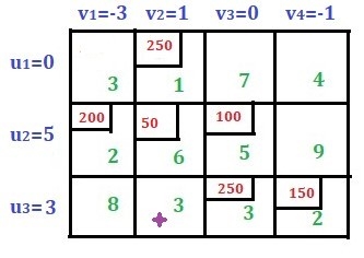
Find the biggest positive penalty here. The maximum value here is 6, which corresponds to cell C21. This cell is now the new base cell. This cell is also included in the solution.
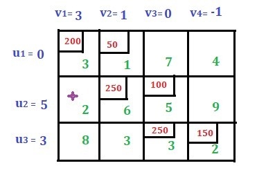
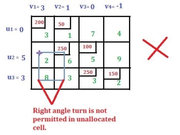
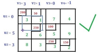
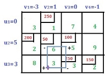
Rules for drawing closed paths or loops. Start with a new base cell and draw a closed path so that only the assigned cell or the new base cell has a right-angle rotation. See the image below.
Assign an alternative plus or minus sign to all cells that bend (or corner) at right angles in the loop, and assign a plus sign to the new base cell.
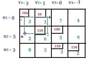
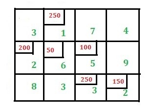
Consider a cell with a negative sign. Compare the assigned values (200 and 250 in this case) and select the minimum value (that is, select 200 in this case). Then subtract 200 from the cells with the minus sign and add 200 to the cells with the plus sign. Then draw a new iteration. Now that we're done with the loop, the new solution looks like this:
Make sure that the total number of allocated cells is equal to (m + n – 1). Again, use the expression ui + vj = Cij to find the u and v values. Where Cij is the cost value for the assigned cell only. Assigning u1 = 0 yields v2 = 1. Similarly, for ui and vj you get the following values:
Use the formula Pij = ui + vj – Cij to find penalties for all unassigned cells.
For C11, P11 = 0 + (-3) – 3 = -6
For C13, P13 = 0 + 0 – 7 = -7
For C14, P14 = 0 + (-1) – 4 = -5
For C24, P24 = 5 + (-1) – 9 = -5
For C31, P31 = 0 + (-3) – 8 = -11
For C32, P32 = 3 + 1 – 3 = 1
There is one positive value. That is, 1 for CNow this cell becomes new basic cell.
Then draw a loop starting from the new base cell. Assign alternative plus and minus signs using the new base cell assigned as a plus sign.
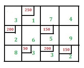
Select the minimum value from the values assigned to the cells marked with a minus sign. Subtract this value from the cell with the minus sign and add it to the cell with the plus sign. The solution now looks like the following image. Check if the total number of allocated cells is equal to (m + n – 1). Find the values of u and v as above.
Now find the penalty for the unallocated cell again, as described above.
When P11 = 0 + (-2) – 3 = -5
When P13 = 0 + 1 – 7 = -6
When P14 = 0 + 0 – 4 = -4
When P22 = 4 + 1 – 6 = -1
When P24 = 4 + 0 – 9 = -5
When P31 = 2 + (-2) – 8 = -8
All penalty values are negative. Therefore, optimality is reached.
Here you find the total cost, that is, (250 * 1) + (200 * 2) + (150 * 5) + (50 * 3) + (200 * 3) + (150 * 2) = 2450.
Q12) Explain Maximum Two Iterations (i.e., Maximum Two Loops) after IFS.
A12) Use Vogel’s method to find an initial basic feasible solution and then find the minimum transportation cost for the following transportation problem by Modi method.
| D1 | D2 | D3 | D4 | Availability |
O1 | 1 | 2 | 1 | 4 | 30 |
O2 | 3 | 3 | 2 | 1 | 50 |
O3 | 4 | 2 | 5 | 9 | 20 |
Requirement | 4 | 40 | 30 | 10 | 100 |
Solution:
Step I: Find the initial basic feasible solution
The initial basic feasible solution obtained by applying Vogel’s approximation method is shown below.
| D1 | D2 | D3 | D4 | Availability | Row Differences |
01 | 1
(20) | 2 | 1
(10) | 4 | 30/10/0 | [0] [0] [1] |
O2 | 3 | 3
(20) | 2
(20) | 1 (10) | 50/40/20/0 | [1] [1] [1] |
03 | 4 | 2
(20) | 5 | 9 | 20/0 | [2] [2] |
Requirement | 20/0 | 40/20/0 | 30/20/0 | 10/0 | 100/100 |
|
Column Differences | [2] [2] | [0] [0] [1] | [1] [1] [1] | [3] |
|
|
Step II Perform Optimality Test
Required number of allocations = m+n-1= 3+4-1 =6=Actual number of allocations. Therefore, optimality test can be performed.
Now, we use Modi for the optimality test.
Now we find the value uj and vj by the relation uj+vj=Cj
For the basic cell (1,1): u1+ v1=1
For the basic cell (1,3): u1+ v3=1
For the basic cell (2,2): u2+ v2=3
For the basic cell (2,3): u2+ v3=2
For the basic cell (2,4): u2+ v4=1
For the basic cell (3,2): u3+ v2=2
Then, let v1=0,then we get
V2 =1; v3=0; v4=-1; u1=1; u2=2; u3=1.Now displaying these values in the table and calculate the cell evaluation.
Iteration 1
Now, subtracting the cell values of the above matrix from the original cost matrix;

Iteration 2
Step III: Since all cell evaluations are positive, the initial basic feasible solution is optimal.
The minimum transportation cost is given by=1x20+1x10+3x20+2x20+1x10+2x20=180.
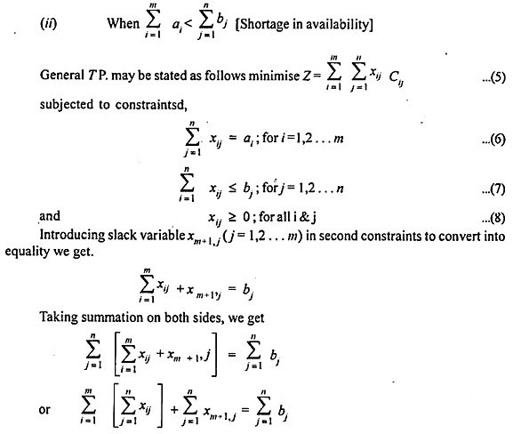
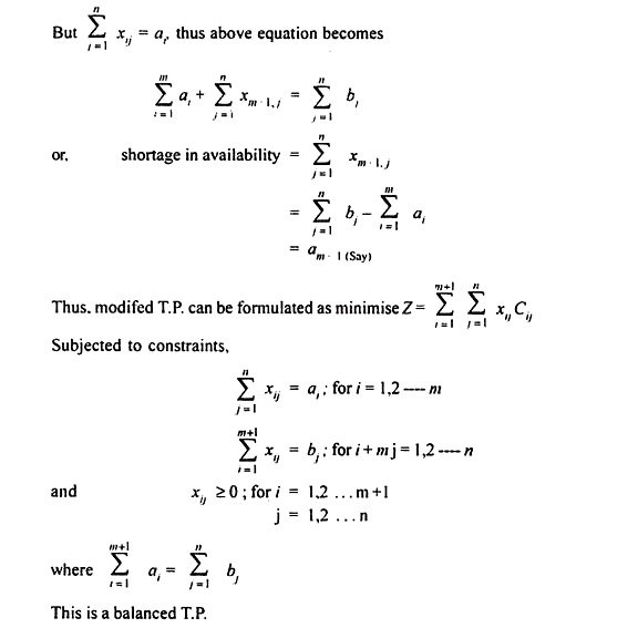
Q13) Write note on Disproportionate transportation problem.
A13) If you have a transportation problem where the sum of the supplies available from all sources is not equal to the sum of the demands of all the destinations, that is, the problem is said to be an imbalanced transportation problem.

However, these imbalanced T.P.S needs to be transformed because the aggregate supply must be equal to the aggregate demand for a viable solution to exist for a well-balanced one.
There are two possibilities:
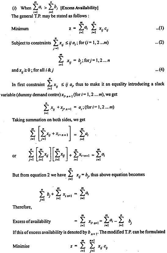
If supply exceeds demand, introduce a dummy demand center (additional destination column) in the transportation problem to absorb the excess supply. The unit cost of shipping cells in this dummy destination column is set to all zeros to represent items that have not been created and sent.

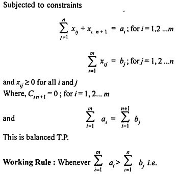
Working rules:
That is, 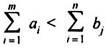 whenever aggregate demand exceeds aggregate supply, we introduce a dummy supply center (additional supply column) in the transportation problem to meet the additional demand. The unit cost of transportation for cells in the dummy row is set to zero.
Second type example:
It solves the transportation problem when the transportation unit price, supply and demand, and supply are as follows.

Solution:
The problem is an imbalanced T.P. because aggregate demand ∑bj = 215 is greater than aggregate supply ∑ai = 195.
Convert this to a balanced T.P by introducing a zero cost dummy origin 04 and giving an equal supply of 215 – 195 = 20 units. Therefore, there is a problem transformed as follows:
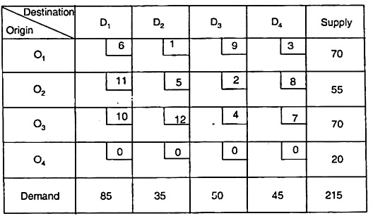
Because of the balance of this issue, there is a viable solution to this issue. Using the lowest cost method, you get the following initial solution:
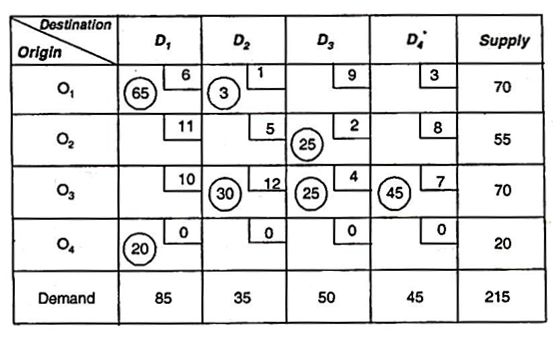
There are seven independent non-negative assignments equal to m + n-1. Therefore, the solution is non-degenerate.
Total shipping cost
= (6 x 65) + (5 x 1) + (30 x 5) + (25 x 2) + (4 x 25) + (7 x 45) + (20 x 0)
= Rs. 1010
To find the best solution:
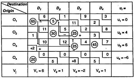
Apply the MODI method steps to the table above.
First, calculate u1 vj&Δij.
Use the cij = ui + vj relationship for the occupied cell
For unoccupied cells, Δij = cij – (ui + vj).
The solution is not optimal because not all Δijs are greater than or equal to zero.
... this cell introduces cells (O3, D1) because the value of Δij is the most negative. Therefore, select this cell as the reference.
For cell O3D1, create a closed path as follows:
O3D1 → O3D3 → O2D3 → O2D2 → O1D2 → OxD1 → O1D1 → O3D3
If you alternate the cycle start (+) of all selected O2D1s with (+) and minus (-) and adjust the associated supply and demand positions, the modified assignments are in the following table.
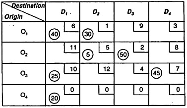
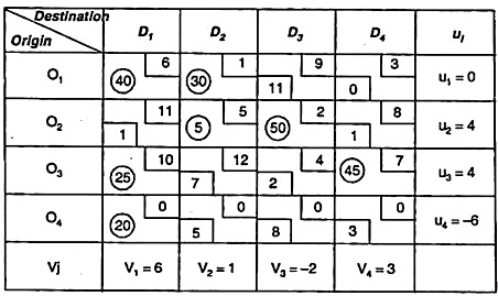
The number of independent allocations is equal to m + n – 1, so check the optimality of this and recalculate ueuj&Δij.
First type example:
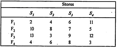
The products are produced in four factories, F1, F2, F3 and F4. Their unit production costs are Rs2, 3, 1, and 5, respectively. The production capacity of the factory is 50, 70, 30 and 50 respectively. Products are supplied to four stores: S1, S2, S3, and S4. The requirements for these stores are 25, 35, 105, and 20, respectively. The transportation unit price is as follows.
Find a transportation plan that minimizes total production and transportation costs.
Solution:
It forms a transport table consisting of both production and transport. cost.
The table is as follows:
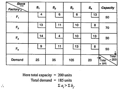
Here, total cost = production unit price + transportation cost
Therefore, the problem is imbalance. Convert to a balanced store by adding a zero cost dummy store S5. Oversupply is given as a rim requirement for this store (220 — 185) = 15 units.
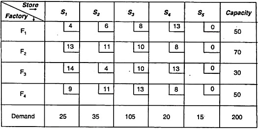
To find the first basic viable solution:
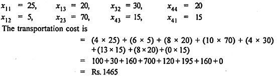
The initial basic feasible solution was obtained by the minimum cost method, and the following initial basic feasible solution was found.
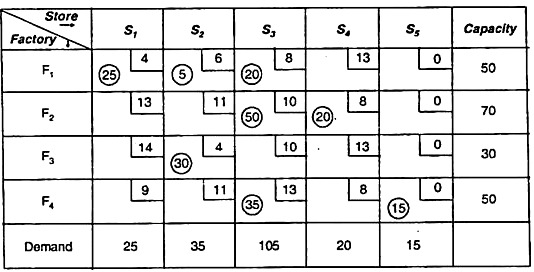
The first basic viable solution that includes a non-negative independent allocation of m + n – 1 = 8. Therefore, the solution is a non-degenerate solution.
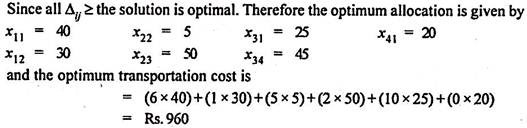
Total shipping cost
= (4 x 25) + (6 x 5) + (8 x 20) + (10 x 50) + (8 x 20) + (4 x 30) + (13 x 35) + (15 x 0)
= Rs. 1525
To find the best solution:
To do this, apply the MODI method to the table above. Since it has an independent non-negative assignment of m + n – 1, we first calculate ui, vj, and Δij with the following relationship:
Occupied cell Cij = ui + vj
Δij = cij – (ui + vj) For unoccupied cells
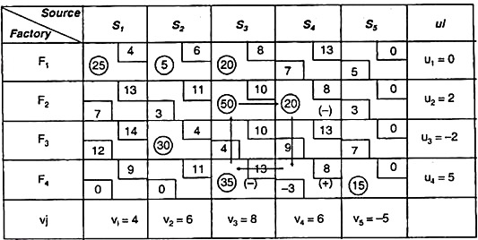
This solution is not optimal because the net rating of cells (F4, S4) is negative. That is, Δ44 = -3
Then draw the closed path from the cell and add it to change the assignment
nd subtraction min = (35,20) = 20.
This closed path is F4S4 → F4S3 → F2S4 → F2S4 → F4S4.
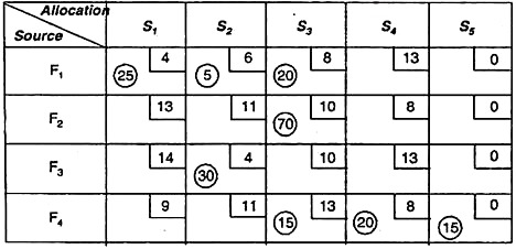
The following table shows this modified assignment.
Again, we are checking the optimality for calculating ui, vj, and Δij.
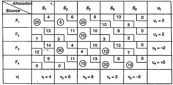
The solution is optimal because all values of Δij ≥ o.
The best solution is
Q14) What is the rule of NWC?
A14) Northwest corner rule
Q15) Define Programming.
A15) Write a function that receives supply and demand. The function updates supply and demand on each iteration, so first copy the arguments and make i and j equal to zero. At each iteration, add 1 to i or j and place the new variable in the resulting list. Crossing all rows and columns returns a basic variable in the form of a tuple containing positions and values.
In [5]:
Defnorth_west_corner (supply, demand):
Supply copy = supply. Copy ()
Demand copy = demand. Copy ()
i = 0
j = 0
bfs = []
Whilelen(bfs) <len(supply) + len(demand) - 1:
s = supply_copy[i]
d = demand_copy[j]
v = min(s, d)
supply_copy[i] -= v
demand_copy[j] -= v
bfs.append(((i, j), v))
ifsupply_copy[i] == 0 and i <len(supply) - 1:
i += 1
elifdemand_copy[j] == 0 and j <len(demand) - 1:
j += 1
returnbfs
In [6]:
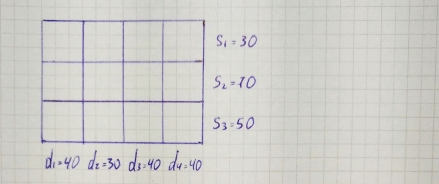
Supply = [30, 70, 50]
Demand = [40, 30, 40, 40]
bfs = north_west_corner (supply, demand)
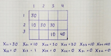
Print (bfs)
[((0, 0), 30), ((1, 0), 10), ((1, 1), 30), ((1, 2), 30), ((2, 2), 10), ((2, 3), 40)]
Q16) Explain Vogel’s Approximation Method (VAM).
A16) The Vogel’s Approximation Method or VAM can be defined as an iterative procedure which is used to find out the initial feasible solution of the transportation problem. The initial basic feasible solution obtained by VAM is either optimal solution or very nearer to the optimal solution. Let’s go through the procedure with an example.
Example:
A mobile phone manufacturing company has three branches which are located in three different regions, say Jaipur, Udaipur and Mumbai. The company is supposed to transport mobile phones to three destinations, say Kanpur, Pune and Delhi. The availability from Jaipur, Udaipur and Mumbai is 40, 60 and 70 units respectively. The demand at Kanpur, Pune and Delhi are 70, 40 and 60 respectively. The transportation cost is shown in the matrix below (in Rs). Use the Vogel’s Approximation Method to find a basic feasible solution (BFS).
Solution:
Step 1: Balance the problem
Balance the problem meaning we need to check that if;
∑ Supply=∑ Demand
If this condition is satisfied, then we will consider the given problem as a balanced problem.
Now, what if it’s not balanced?
i.e., Σ Supply≠Σ Demand
If such a condition occurs, then we have to add a dummy source or market; whichever makes the problem balanced.
Step 2: Find out the Row difference and the Column difference
Now, we will find out the row and the column difference of the provided matrix.
For the same we will solve this as follows:
Here as you can see in the first row, we need to find out cell containing smallest value (least cost), and the second least.
Hence, we find 1 and 4 as the two lowest values in the first row.
Take the difference of these two numbers, i.e. (4−1)=3.
In a similar manner, find out differences for all the rows as shown above.
The same procedure is to be done with columns.
So, for the first column, you will get, (4−3)=1.
Find out difference for all columns as done above.
Step 3: Select the row/column with highest difference
As we can see above, the highest difference value is 4 which is for the last row.
So we will select that row, and find out the minimum cost in that row.
You will find that, minimum cost is 2.
Now, compare the supply and demand for this row and column respectively.
We find that, we have supply as 70 and demand as 40 for the selected cell.
Compare both and select the minimum of them for the allocation in the cell, as shown below.
Cross out the column whose demand is fulfilled.
Step 4: Remove the row/column whose supply or demand is fulfilled and prepare new matrix and repeat the same procedure

As it can be seen, we now have a new matrix with second column removed (as its demand was 40 which was fulfilled)
Now, we will repeat the same procedure until we're done with all allocations.
i.e.,


Step 5: After all the allocations are completed, write all the allocations in the matrix and find Transportation cost
We have all allocations with their respective cell now.
Find transportation cost as follows:
Transportation cost= (1x40)+(3x40)+(3x20)+(6x30)+(2x40)=Rs 480.
Q17) What is the two steps to solve transportation problem?
A17) There are two steps to solving a transportation problem. The first phase requires finding the first basic viable solution, and the second phase optimizes the first basic viable solution obtained in the first phase. There are three ways to find the first basic viable solution.
This article describes how to optimize your first basic viable solution through the examples provided. Consider the following transportation problem.
Q18) What do you mean by Optimal solution?
A18) An Assignment problem may have more than one optimal solution, which is called multiple optimal solutions. Multiple optimal solutions mean thatthe total cost or total profit will remain same for different sets or combinations of allocations.It is sometimes seen that a certain task cannot be performed by a person or a machine. A restricted assignment problem is the one in which one or more allocations are prohibited or not possible. The solution should be found taking into consideration these restrictions. For such allocations we assign “M”, which is infinitely high cost. No allocation is given in M.
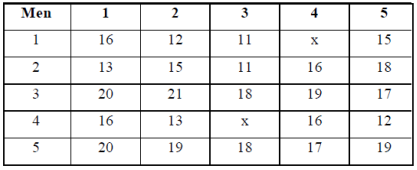
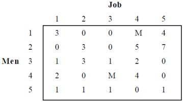
Example: Five jobs are to be assigned to five men. The cost (in Rs.) of performing the jobs by each man is given in the matrix. There are restrictions in the assignment that Job 4 cannot be performed by Man 1 and Job 3 cannot be performed by Man 4. Find the optimal assignment of job and its cost involved.
Assignment Problem
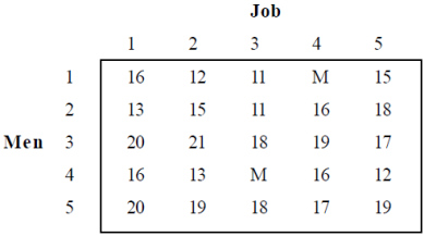
Solution: Assign a large or infinite value to the restricted combinations or introduce ‘M’, see table.
Large Value Assignment to Restricted Combinations
Reducing the matrix row-wise
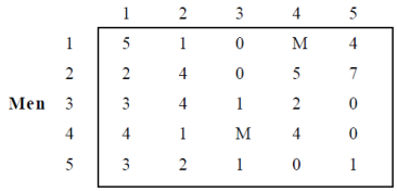
Reducing the matrix column-wise
Draw minimum number of lines so as to cover all zeros, see Table below.
All Zeros Covered
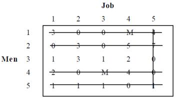
Now, number of lines drawn = Order of matrix, hence optimality is reached.
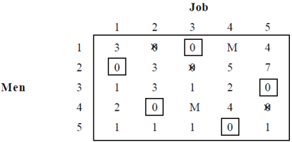
Allocating Jobs to Men.
Job Allocation to Men
Q19) Define allocation problem.
A19) Allocation problems are specific cases of transportation problems where the goal is to allocate an outsized number of resources to an equivalent number of activities so as to attenuate the entire cost or maximize the entire profit of the allocation.
Allocation issues arise because available resources like men, machines, etc. have different degrees of efficiency for performing different activities. Therefore, there are different costs, benefits, or losses to perform different activities.
Definition of assignment problem:
Suppose you've got n jobs to run and n people can run these jobs. Efficiency varies, but assumes that every person can run each job in just one occasion period. However, if the i-th person is assigned to the j-th job, cij are going to be the value. The matter is finding an assignment (which job should be assigned to which person on a one-to-one basis). This sort of problem is understood as an allocation problem in order that the entire cost of running all jobs is minimized.
Q20) What are the steps to solve the allocation problem?
A20) The Hungarian allocation method provides an efficient thanks to find the simplest solution without having to match all the solutions directly. It works on the principle of reducing a given cost matrix to a chance cost matrix.
Opportunity cost indicates the relative penalty related to allocating resources to an activity, instead of allocating the simplest or least cost. Optimal allocation are often achieved if a minimum of one zero in each row and column can reduce the value matrix to some extent.
The Hungarian method are often summarized within the following steps.
Step 1: Create a price table from the given problem.
If the amount of rows isn't adequate to the amount of columns, or the other way around, you would like to feature dummy rows or columns. The value of allocating dummy cells is usually zero.
Step 2: Find the chance Cost Table:
(A) Find the littlest element in each row of the required cost table and subtract it from each element therein row.
(B) Within the reduction matrix obtained from 2 (a), find the littlest element in each column and subtract it from each element. Each row and column has a minimum of one zero value.
Step 3: Make an allocation within the cost Matrix:
The allocation procedure is as follows:
(A) Examine the rows continuously until you get a row with just one unmarked zero. Make the assignment one zero by creating a square around it.
(B) For every zero value assigned, delete (cancel) all other zeros within the same row and / or column.
(C) Repeat steps 3 (a) and three (b) for every column, leaving just one unassigned zero value.
(D) If there are two or more unmarked zeros within the rows and / or columns and therefore the check cannot select one, select any assigned zero cell.
(E) Continue this process until all zeros within the matrix are enclosed (assigned) or deleted (x).
Step 4: Optimal criteria:
If the assigned cell members are adequate to the row sequence that is the best solution. The entire cost related to this solution is obtained by adding the first cost figure to the occupied cell.
If zero cellsare arbitrarily selected in step (3), an alternate optimal solution exists. However, if you can't find the simplest solution, attend step (5).
Step 5: Modify the chance cost table.
Use the subsequent procedure to draw a group of horizontal and vertical lines that cover all zeros within the revised cost table obtained in step (3).
(A) Add a check (√) to every row that has not been assigned.
(B) Examine the marked line. If zeros occur in these columns, check each row that contains the assigned zeros.
(C) Repeat this process until you'll not mark rows or columns.
(D) Draw a line through each marked column and every unmarked row.
If the amount of drawn lines is adequate to the amount (or columns), then the present solution is that the best solution otherwise, attend step 6.
Step 6: Create a newly revised cost Table.
(A) Select the littlest element from the cells that aren't covered by the road, and call this value K.
(B) Draw K from all the weather within the cell that isn’t covered by the road.
(C) Add K to the element within the cell covered by the 2 lines, that is, the intersection of the 2 lines.
(D) The weather of the cell covered by one row aren't changed.
Step 7: Repeat steps 3-6 close up the lights for the simplest solution