UNIT 2
Consumer Behaviour
Q1) Explain indifference curve analysis
A1) Indifference curve analysis
Utility analysis suffers from a flaw in the subjective nature of utility, that is, the inability to measure utility quantitatively and accurately. To overcome this difficulty, economists developed a different approach based on the indifference curve. According to this indifference curve analysis, utility cannot be accurately measured, but the consumer can state which of the combinations of two goods he prefers, without describing the magnitude of the strength of his preference. This means that if the consumer is presented with a number of different combinations of goods, he can order or rank them on a “scale of preference “if the different combinations are marked a, B, C, D, E, etc. In this case, the consumer can tell whether he likes A to B or B to A or is indifferent between them. Similarly, he can show his preference or indifference between other pairs or combinations. The concept of order utility means that consumers cannot go beyond stating their preferences or indifference. In other words, if consumers prefer A to B, they don't know by “how much “they prefer A to B. Consumers cannot state the “quantitative difference “between different satisfaction levels. He can simply compare them “qualitatively". That is, it is possible to determine whether simply one satisfaction is higher than another, or lower, or equal.
The basic tool of the Hicks-Allen order analysis of demand is the indifference curve, which represents all those combinations of goods that give the consumer the same satisfaction. In other words, all the combinations of goods that lie on the consumer's indifference curve are equally preferred by him. The independence curve is also known as the Iso-utility curve. Indifferent schedules are tabular statements showing different combinations of two goods that bring the same level of satisfaction.
Table 2.4 Indifference schedule
Combination Rice (X) Wheat (Y)

I | 1 | 12 |
II | 2 | 8 |
III | 3 | 5 |
IV | 4 | 3 |
V | 5 | 2 |
Now consumers are asked to tell the amount of wheat (Y) they are willing to give up the benefit of an additional unit of rice (X) so that the level of satisfaction remains the same. If the profit of one unit of rice fully compensates for the loss of 4 units of wheat, then the following combination of 2 units of rice
And eight units of wheat will give him as much
Satisfaction as the first or first combination. A set of indifferent curves representing the size of preference at different levels of satisfaction are understood because the indifferent curve map (figure 2.3).
Although the combination lying on the indifferent curve 3 (IC3) provides the same satisfaction
Product X

Commodity X
Fig 2.3 Indifference Curve Map
Figure 2.3 indifference curve map
The level of satisfaction in the indifference curve 3 (IC3) is greater than the level of
Satisfaction with indifference curve 2(IC2).
I) The nature of the indifference curve
A) Downward inclination: the indifference curve tilts downwards from left to right.
This means that when the amount of one good in a combination increases, the amount of another must necessarily be reduced so that the total satisfaction is constant.
If the indifference curve is a horizontal straight line (parallel to the X-axis),
Then the indifference curve is a horizontal straight line (parallel to the X-axis),
As shown in the figure. 2.4 (a) means that as the amount of good X increases,
The amount of good Y will remain constant, but the consumer will remain
Indifferent among the various combinations.
This cannot be done, because consumers always prefer
A large amount of good to a small amount of its good.
Similarly, the indifference curve cannot be a vertical straight line


 Commodity X Commodity X Commodity X
Fig.2.4 (a) Horizontal Fig.2.4 (b) Vertical Fig.2.4(c) Upward Sloping
Indifference Curve Indifference Curve Indifference Curve
A vertical straight line means that while the amount of good y in combination increases the amount of good X remains constant. The third possibility for the curve is to lean upward to the right.
Q2) Explain budget line
A2) Knowledge of the concept of budget lines is important for understanding the idea of consumer equilibrium. The higher apathy curve shows higher satisfaction than the lower one. Therefore, the consumer in his attempt to maximize his satisfaction will try to reach the highest possible indifference curve.
However, in order to buy more goods and seek to get more satisfaction, he must work under two constraints; firstly, he must pay the price of the goods, and secondly, he has a limited money income to buy the goods. Therefore, how far he will go for his purchase depends on the price of the goods and the income of the money he will have to spend on the goods.
Now, in order to explain the equilibrium of consumers, it is also necessary to introduce into the indifferent diagram a budget line, which represents the price of goods and the income of consumers ' money.
Suppose that our consumers have Rs income. Let's say Rs the price of a good X in the market to spend on 50 goods X and Y. That of 10 and Y Rs per unit. 5 per unit if the consumer spends his entire income of Rs. In a good X 50,he would buy 5 units of X;if he spent his entire income of Rs. To 50 good Y he would buy 10 units of Y if a straight line connecting 5X and 10Y is drawn, we get what is called a price line or budget line.
This budget line looks at all the figures of two goods a consumer can buy by spending his given money income on two goods at a given price. 8.14 show it in Rs. The price of 50 and X and Y is Rs. 10 and Rs. 5 respectively consumers can buy 10Y and OX, or 8Y and IX;or 6Y and 2X, or 4Y and 3x etc.
In other words, he can buy any combination that is on the budget line at the given price of the goods with the income of his given money. It should be noted that the combination of goods as H (5Y and 4x) above and outside the given budget line is beyond the reach of consumers.
However, a combination that is within the budget line, such as k (2X and 2Y), is within the reach of die consumer, but buying such a combination will not spend all the proceeds of the Rs. 50. Therefore, on the assumption that the totality of the given income will be spent on the given goods and at the given price, the consumer must choose from all the combinations that are on the budget line. It is also clear that over budget lines give a graphical budget. The combination of goods to the right of the budget line is unattainable, since the consumer's income is not enough to be able to buy those combinations. Given his income and the price of goods, the combination of goods on the left side of the budget line is achievable, that is, the consumer can buy any of them.
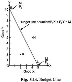
It is also important to remember that it is an intercept OB on the Y-axis in the figure. 8.14 is OB=M/Py, equal to the amount of his overall income divided by the price of goods Y. Similarly, The Intercept OL on the x-axis measures the total revenue divided by the price of the product X.OL=M / Vx. Where Px and Py represent the price of goods X and Irrespectively, and M represents the income of money. The above budget line formula (8.1) means that given the consumer's money income and the price of two goods, all the combinations lying on the budget line will cost the same amount and can therefore be purchased at a given income. A budget line can be defined as a set of a combination of two goods that can be purchased if the whole of a given income is spent on them and its slope is adequate to the negative of the worth ratio.
Budget space:
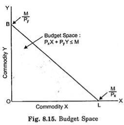
It is necessary to carefully understand that the budget equation PxX+PyY=M or Y=M/Py–Px/Py. X is indicated by the budget line in the figure. 8.14 only describe budget lines, not budget spaces. Budget space indicates a set of combinations of all goods that can be purchased by spending all or part of the given income. In other words, budget space represents all those combinations of goods that consumers can afford to buy, given budget constraints.
Thus, the budget space implies a set of all combinations of two goods in which the income spent on Good X (i.e., Px X) and the income spent on good Y (i.e., PyY) must exceed the monetary income given.
Thus, we can algebraically represent the budget space in the following form of the inequality:
Pxx+PyY PxX+PyY
The budget space is graphically shown in the diagram. 8.15 as a shaded area. Budget space is the entire area bounded by the budget line BL and two axes.
Changes in Price and Shift in Budget Line:
Now, what happens to the worth line when the worth of the products changes or the income changes. First, let’s take the case of a change in the price of goods. This is shown in the figure. 8.16. Suppose that the first budget line is BL, given a certain price of goods X and Y and a certain income. Suppose that the price of X falls, and the price and income of Y remain unchanged.
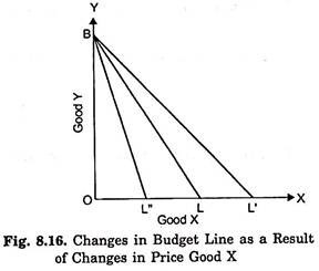
Now, with the lower price of X, the consumer will be able to buy X in greater quantities than before with his given income. Let at the lower price of X, the given income is greater than OL'X to buy OL'. Since the price of Y will remain the same, there will be no change in the purchase volume of good Y with the same given income and there will be no shift to point B as a result. Therefore, if the price of good X falls, the income of consumers 'money and the price of Y remain constant, the price line will take a new position BL'.
Now, what happens to the budget line (initial budget line BL) if the price of good X rises and the price and income of good Y remain unchanged. At a higher price for a good X, consumers can buy a smaller amount of X than before. Therefore, with the increase in the price of X, the price line is assumed to be a new position BL".
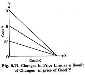
It is a fig. 8.17 indicates the change in the price line when the price of good Y falls or rises, while the price and income of X remain the same. In this case, the initial budget line is BL.A good y price decline, while others remain unchanged, consumers can buy a lot of y with a given money income, thus the budget line will shift to LB', as well as the price y rise, when others are constant, the budget line will shift to LB'.
Changes in income and shifts in budget lines:
Now, the question is what happens to the Y line of the budget if the income changes, while the price of the goods remains the same. The figure shows the effect of changes in income on the budget line. 8.18. Given the specific price of goods and income, let BL be the initial budget line."When a consumer's income increases while the prices of both goods X and Y have not changed, the price line shifts upwards (for example, to B'l') and parallel to the original budget line BL, which means that when income increases, if the whole of income is spent on X, consumers can buy a proportionately greater amount of good X than before, and the whole of income is spent on Y. this is because it is possible to buy a good y in a proportionately larger amount than before. On the other hand, when a consumer's income decreases, the price of both commodity X and commodity X decreases.
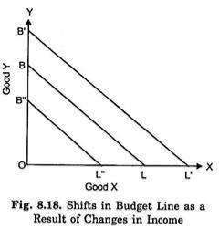
Y remains unchanged, the budget line shifts downward (for example, to B"L"), but remains parallel to the original price line BL. This means that if the whole of the income is spending a change in the income relative to X, if the whole of the income is spending a change in the income relative to X, then the whole of the income is spending a change in the income relative to X.
From above it is clear that the budget line changes when the price of goods changes or the income of consumers changes.
Therefore, the two determinants of the budget line are:
(a) The price of the goods, and
(b) The consumer's income spent on goods;
Two commodity budget lines and price slope:
It is also important to recollect that the slope of the budget line is adequate to the ratio of the worth of two goods. This can be proved with the help of figures. 8.14. Suppose that the given income of the consumer is M, and the given price of the goods X and Y are Px and Py, respectively. The budget line slope BL is OB / OL. I'm going to prove that the slope OB/OL is equal to the ratio of the price of the goods X and Y.
If the whole of the given income M is spent on it, then the amount of good X purchased is OL.

Now, the amount of good Y purchased if the whole of the given income M is spent on it is OB.


Therefore, it has been proven that the slope of the budget line BL represents the ratio of the price of two goods.
Q3) Explain consumer equilibrium
A3) You are now clear about the indifference curve and budget lines. Next, let's look at the consumer equilibrium. Consumers are in equilibrium when they get maximum satisfaction from the goods and are not in a position to rearrange their purchases. There is a defined apathy map showing the scale of consumer preferences across different combinations of two goods X and Y.
Consumers have a fixed income and want to spend it entirely on goods X and Y.
The price of goods X and Y is fixed to the consumer.
The goods are homogeneous and divisible.
The consumer acts rationally and maximizes his satisfaction.
Consumer equilibrium
Take his indifference curve and budget line together to show the combination of two goods X and Y that consumers buy to be balanced.
We know,
Indifferent map-shows the scale of consumer preferences between various combinations of two goods
Budget line-he shows his money income and various combinations that can afford to buy at the price of both goods.
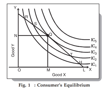
The following figure shows the indifference map with 5 indiscriminate curves (ic1, IC2, IC3, IC4, and IC5) and the budget lines PL for good X and good Y. In order to maximize his level of satisfaction, the consumer tries to reach the highest indifference curve. We assume budget constraints, so he will be forced to stay on the budget line.
So, what kind of combination is it?
Let's say he chose the combination R from the figure. 1, we see that R is on the low indifference curve–IC1. He can easily afford the combination S, Q, or T that is on a high Ic. Even if he chooses the combination H, the argument is similar because H is on the curve IC1.
Next, let's check out the mixture S lying on the curve IC2. Again, he can reach a better level of satisfaction within the budget by choosing the mixture Q lying on IC3–the argument is analogous for the mixture T, since the higher T is also on the curve IC2.
Therefore, we have left the combination Q.
What happens when he chooses the combination Q?
This is the simplest choice because Q is on his budget line and pts puts him on the simplest possible indifference curve, IC3. There are higher curves, IC4 and IC5, but they are over his budget. Thus, he reaches equilibrium at the point Q on the curve IC3.
Note that at this point the budget line PL is bordered by the indifference curve IC3. Also in this position, consumers buy X in OM amount and Y in ON amount.
Since Point Q is tangent, the slope of line PL and curve IC3 is equal at this point. In addition, the slope of the indifference curve shows that the substitution limit rate (MRSxy) of X with respect to Y is
Hence, at the equilibrium point Q,
MRSxy = MUxMUyMUxMUy = PxPy
Also, the slope of the price line (PL) shows the ratio of X and Y prices. Therefore, we can say that the consumer equilibrium is achieved when the price line is bordered by the indifference curve. Alternatively, when the substitution limit rate of goods X and Y is equal to the ratio between the prices of two goods.
Q4) Explain consumer surplus
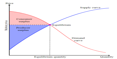
A4) Consumer surplus is the difference between the maximum price a consumer is willing to pay and the actual price they do pay. If a consumer would be willing to pay more than the current asking price, then they are getting more benefit from the purchased product than they spent to buy it. Consumer surplus plus producer surplus equals the total economic surplus in the market.
This chart graphically illustrates consumer surplus in a market without any monopolies, binding price controls, or any other inefficiencies.. This means that the price could not be increased or decreased without one of the parties being made worse off. The consumer surplus, as marked in red, is bound by the y-axis on the left, the demand curve on the right, and a horizontal line where y equals the equilibrium price. This area represents the amount of goods consumers would have been willing to purchase at a price higher than the optimal price. Generally, the lower the price, the greater the consumer surplus.
Q5) Explain concept of demand
A5) Concept of demand
Ordinarily, DEMAND means a desire or want for something. In economics, however, demand means much more than that. Economics attach a special meaning to the concept of demand i.e. ‘Demand is the desire or want backed up by money.’ It means effective desire or want for a commodity, which is backed up the purchasing power and willingness to pay for it.
Demand, in economics, means effective demand for a commodity. It requires three conditions on the part of consumer.
In short,
Demand = Desire + Ability to pay + Willingness to spend
Demand is always related to Price & Time. Demand is not the absolute term. It is a relative concept. Demand for a commodity should always have a reference to Price & Time.
 For e.g. – Price Grapes for house hold at a price of Rs. 20/- per Kg., Rs. 10/- per Kg
 Time per day, per month, per year
Definition:
The Demand for a commodity refers to the quantity of a commodity that a person is willing to buy at different prices during period of time.
Q6) Explain concept of supply
A6) Supply is the willingness and ability of producers to produce goods and services and make it available to the consumers. The total amount of goods and services available for purchases at any specific price.
Definition: Supply is an economic term that refers to the amount of a given product or service that suppliers are willing to offer to consumers at a given price level at a given period.
Determinants
For example, if the price of tea increases, farmers would tend to grow more tea than coffee. This would decrease the supply of tea in the market.
Q7) Explain law of demand
A7) The law of demand states that all other factors remain constant or equal, an increase in the price causes a decrease in the quantity demanded and a decrease in goods or services price leads to increase in the quantity demanded. Thus it expresses an inverse relationship between price and demand.
For example, at Rs 70 per kg consumer may demand 2 kg of apple. On the other hand, the price rises to 100/- per kg then he may demand 1 kg of apple
Assumption of law of demand
Given these assumption, the law of demand is explained in the below table –
Price(Rs) | Quantity demanded |
10 | 10 |
8 | 20 |
6 | 30 |
4 | 40 |
2 | 50 |
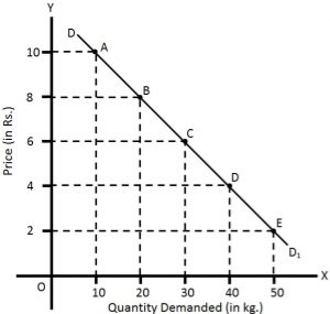
The above table shows that when the price of apple, is Rs. 10 per kg, 10 kg are demanded. If the price falls to Rs.8, the demand increases to 20 kg. Similarly, when the price declines to Rs 2, the demand increases to 50 kg. This indicates the inverse relation between price and demand.
Also, in the above figure the demand curve slopes downwards as the price decreases, the quantity demanded increases.
Exception of law of demand
Under the following circumstances, consumers buy more when the price of a commodity rises, and less when price falls which leads to upward sloping demand curve.
Q8) Explain Movement vs. shift in the demand curve
A8) Definition of Movement in Demand Curve
Movement along the demand curve depicts the change in both the factors i.e. the price and quantity demanded, from one point to another. Other things remain unchanged when there is a change in the quantity demanded due to the change in the price of the product or service, results in the movement of the demand curve. The movement along the curve can be in any of the two directions:
Upward Movement: Indicates contraction of demand, in essence, a fall in demand is observed due to price rise.
Downward Movement: It shows expansion in demand, i.e. demand for the product or service goes up because of the fall in prices.
Hence, more quantity of a good is demanded at low prices, while when the prices are high, the demand tends to decrease.
Definition of Shift in Demand Curve
A shift in the demand curve displays changes in demand at each possible price, owing to change in one or more non-price determinants such as the price of related goods, income, taste & preferences and expectations of the consumer. Whenever there is a shift in the demand curve, there is a shift in the equilibrium point also. The demand curve shifts in any of the two sides:
Rightward Shift: It represents an increase in demand, due to the favourable change in non-price variables, at the same price.
Leftward Shift: This is an indicator of a decrease in demand when the price remains constant but owing to unfavourable changes in determinants other than price.
Basis for comparison | Movement in demand curve | Shift in demand curve |
Meaning | Movement in the demand curve is when the commodity experience change in both the quantity demanded and price, causing the curve to move in a specific direction. | The shift in the demand curve is when, the price of the commodity remains constant, but there is a change in quantity demanded due to some other factors, causing the curve to shift to a particular side. |
What is it | Change along the curve | Change in the position of the curve. |
Determinant | Price | Non price |
Indicates | Change in Quantity Demanded | Change in demand |
Result | Demand Curve will move upward or downward. | Demand Curve will shift rightward or leftward. |
Q9) Explain Elasticity of demand – Price, Income and cross elasticity
A9) Under law of demand, price falls and demand rises, vice versa. But how much the quantity rise or fall for a given change in price is not determined in law of demand. So the concept of elasticity of demand is derived to know how much quantity demanded changes for a change in the price of goods or services.
“The elasticity (or responsiveness) of demand in a market is great or small according as the amount demanded increases much or little for a given fall in price, and diminishes much or little for a given rise in price”. – Dr. Marshall.
Elasticity means sensitivity of demand to the change in price.
The formula for calculating elasticity of demand is:
EP = proportional changes in quantity demanded/proportional changes in price
Types of elasticity of demand
Elasticity of demand is of following types
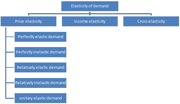
Price of elasticity of demand –
- Ep = percentage change in quantity demanded/percentage change in price
There are 5 types of price elasticity of demand given below
- A small change in price results to major change in demand is said to be perfectly elastic demand
- The demand curve in perfectly elastic demand represent horizontal straight line
- Ep = infinity
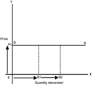
From the above figure, we can see at price P1 consumers are ready to buy as much quantity as they want. A slight increase in price may result to fall in demand to zero.
2. Perfectly inelastic demand


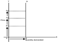
From the above fig, we can see that price is rising from P1 to P2 to P3, but there is no change in the demand. This cannot happen in practical situation. But, in essential goods such as salt, with the change in price the demand does not change.
3. Relatively elastic demand
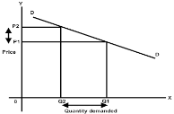

4. Relatively inelastic demand

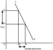
5. Unitary elastic demand
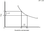
In the above figure we can observe that proportionate change in price from P to P1 cause the same proportionate change in price from M to M1
Income elasticity demand
The income elasticity is measures the sensitivity of quantity demanded for a goods or services to a change in consumer’s income
 Formula - Percentage change in the quantity demanded
Percentage change in the consumer’s income
Types
When a proportionate change in the income of a consumer increases the demand for a product and vice versa, income elasticity of demand is said to be positive. In case of normal goods, the income elasticity of demand is generally found positive.
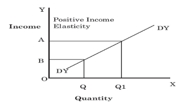
In Figure, DYDY is the curve representing positive income elasticity of demand. The curve is sloping upwards from left to the right, which shows an increase in demand (OQ to OQ1) as a result of rise in income (OB to OA).
2. Negative income elasticity of demand –
When a proportionate change in the income of a consumer results in a fall in the demand for a product and vice versa, income elasticity of demand is said to be negative. In case of inferior goods, the income elasticity of demand is generally found negative.
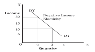
In Figure, DYDY is the curve representing negative income elasticity of demand. The curve is sloping downwards from left to the right, which shows a decrease in the demand as a result of a rise in income. As shown in Figure, with a rise in income from 10 to 30, the demand falls from 3 to 2.
3. Zero income elasticity of demand –
When a proportionate change in the income of a consumer does not bring any change in the demand for a product, income elasticity of demand is said to be zero. It generally occurs for utility goods such as salt, kerosene, electricity.
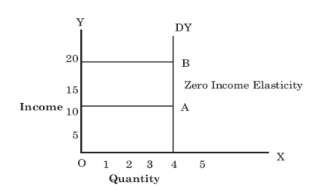
In Figure, DYDY is the curve representing zero income elasticity of demand. The curve is parallel to Y-axis that shows no change in the demand as a result of a rise in income. As shown in Figure, with a rise of income from 10 to 20, the demand remains the same i.e. 4.
Cross elasticity
“The cross elasticity of demand is the proportional change in the quantity of X good demanded resulting from a given relative change in the price of a related good Y” Ferguson
It measures the percentage change in the quantity demanded of commodity X to the percentage change in the price of its substitute/complement Y
 Formula – proportionate change in quantity demanded of X
Proportionate change in the price of Y
Types
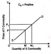
In the above figure, at price OP of Y-commodity, demand of X-commodity is OM. Now as price of Y commodity increases to OP1 demand of X-commodity increases to OM1 Thus, cross elasticity of demand is positive.
2. Negative - A proportionate increase in price of one commodity leads to a proportionate fall in the demand of another commodity because both are demanded jointly refers to negative cross elasticity of demand.
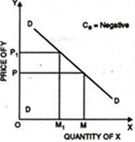
When the price of commodity increases from OP to OP1 quantity demanded falls from OM to OM1. Thus, cross elasticity of demand is negative.
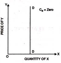
3. Zero - Cross elasticity of demand is zero when two goods are not related to each other. For instance, increase in price of car does not effect the demand of cloth. Thus, cross elasticity of demand is zero.
Q10) Explain factors affecting elasticity of demand.
A10) Factors affecting elasticity of demand
(i) Availability of close substitutes: Demand for a commodity which has large number of substitutes, is usually more elastic than those commodities which have no substitutes. For example, coke, Pepsi, Limca etc. are good substitutes. Even a small rise in price of coke will induce the buyers to go for its substitutes. On the other hand demand for electricity will be less elastic because it has no close substitutes.
(ii) Nature of the Commodity: Demand for necessities like medicines, food grains is less elastic because we have to consume them in minimum required quantity, whatever their price may be. But demand for comforts and luxuries like refrigerators, air conditioners etc. is more elastic because their consumption may be postponed for future if their price rises.
(iii) Share in Total Expenditure: Greater the proportion of income spent on the commodity, more is the elasticity of demand for it. Demand for a commodity is inelastic if proportion of income spent on that commodity is very small.
(iv) Level of Price: Demand for a commodity at higher level of price (like air conditioners, cars etc.) is generally more elastic than for a commodity at lower level of price (like match box, pencils etc.)
(v) Level of Income: Demand for a commodity is generally less elastic for higher income level groups in comparison to people with low incomes. For example, if price of a good rises, a rich consumer is not likely to reduce his demand but a poor consumer can reduce his demand for that commodity.
(vi) Habits: Habits of consumers also determine price elasticity of demand of commodities. For example, a chain smoker will not restrict his smoking even when the prices of cigarettes rise.