UNIT 3
Production
Q1) Explain factors of production
A1) The primary purpose of economic activity is to produce utility for individuals. Business firm are the important component of the economic system. The business firm purchase the factors of production such as land , labour, capital, etc from households , other business firm and government to produce different goods and services which it sells to its customers.
Definition
According to Bates and Parkinson:
“Production is the organized activity of transforming resources into finished products in the form of goods and services; the objective of production is to satisfy the demand for such transformed resources”.
Factors of production
Production of a commodity requires the use of certain factors of production. Factors of production transforms those resources into different goods or services which is made available to the end user
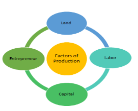
Classification of factors of production
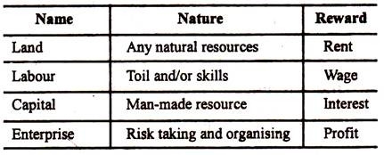
“Land in economics is taken to mean not simply that part of the earth’s surface not covered by water, but also all the free gifts of nature’s such as minerals, soil fertility, as also the resources of sea. Land provides both space and specific resources”.
Characteristics
). But today much of the services of land require expenditure to maintain them.
Return
The income received by the owner of land is called rent. Rent paid is more than the use of land. It also included payment of other factors which involves in making the resources available to the end user.
2. Labour
According to Marshall, “Any exertion of mind or body undergone partly or wholly with a view to some good other than the pleasure derived directly from the work is called labor.”
Characteristics
Return
The reward paid in return for the services of labour is called as wage or salary. Supply of labour depends on their wages. Increase in wages will lead to increase in supply of labour.
3. Capital
‘Produced means of production.’
Characteristics
Return
The earning of capital is known as interest. It is the sum paid by the borrower to the lender who needs finance to purchase capital equipment
4. Enterprise
An entrepreneur is a person, who undertakes risks, mobilizes resources, and generates employment by establishing and running an enterprise.
Characteristics
Return
The return to the entrepreneur is profit. Profit is the reward for successful conduct of business.
Q2) Explain law of variable proportion
A2) Law of variable proportion
The law of variable proportion states that keeping all other factors fixed, when the quantity of one factor increased, the marginal product of that factor will eventually decline. This means that upto the use of a certain amount of variable factor, marginal product of the factor may increase and after a certain stage it starts diminishing. When the variable factor becomes relatively abundant, the marginal product may become negative.
Definition
“As the proportion of the factor in a combination of factors is increased after a point, first the marginal and then the average product of that factor will diminish.” Benham
Assumption
The following assumption of law of variable proportion
Illustration of the Law:
The law of variable proportion is explained in the below given table and figure. Assume that a there is a given fixed amount of land, in which more labour (variable factor) is used to produce agricultural product.
Units of labour | Total product | Marginal product | Average product |
1 | 2 | 2 | 2 |
2 | 6 | 4 | 3 |
3 | 12 | 6 | 4 |
4 | 16 | 4 | 4 |
5 | 18 | 2 | 3.6 |
6 | 18 | 0 | 3 |
7 | 14 | -4 | 2 |
8 | 8 | -6 | 1 |
In the above table we can observe that upto the use of 3 units of labour, total product increases at an increasing rate. But after the third unit total product increases at a diminishing rate.
A marginal product is the incremental change in total product as a result of increasing the variable factor i.e labour. We can see from the table, marginal product of labour initially rises and beyond the use of third unit it starts diminishing. The use of 6 units does not add anything in the production. Thus marginal product of labour fallen to zero. After the 6 unit, total product decreases and marginal product becomes negative.
Average product is derived by dividing total product by the quantity of variable unit. Till the 3 unit of labour, average product increases. Whereas after the 3 unit, average product is falling throughout.
Three Stages of the Law of Variable Proportions:
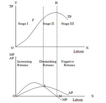
The stages are discussed in the below figure where labour is measured on the X-axis and output on the Y-axis.
Stage 1. Stage of Increasing Returns:
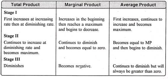
In this stage, total product increases at an increasing rate till point F..ie the curve TP concave upwards upto point F which means marginal product of labour rises. Because efficiency of fixed factor increases with the increase in variable facto labour. After point F, the total product starts increasing at a diminishing rate. Looking at the next figure, marginal product of labour is maximum, after which it diminishes. This stage is called the stage of increasing returns because the average product of the variable factor labour increases throughout this stage. This stage ends at the point where the average product curve reaches its highest point.
Stage 2. Stage of Diminishing Returns:
The stage 2 ends, when the total product increases at a diminishing rate until it reaches it maximum point H. In this stage both marginal product and average product are diminishing but remain positive. Because fixed factor land becomes inadequate with the increase in the quantity of variable factor labour. At point M marginal product is zero which corresponds to the maximum point H of the total product curve.
Stage 3. Stage of Negative Returns:
In stage 3, with the increase in variable factor labour, the total product decline. Therefore the TP curve slopes downward. As a result, marginal product of labour is negative and MP cure falls below x axis. In this case fixed factor land becomes too much inadequate to the increase in variable factor labour.
Q3) Explain returns of scale
A3) Return of scale
In long run, no factors are fixed. Return of scale refers to proportionate change in productivity from proportionate change in all the inputs.
Definition:
“The term returns to scale refers to the changes in output as all factors change by the same proportion.” Koutsoyiannis
“Returns to scale relates to the behaviour of total output as all inputs are varied and is a long run concept”. Leibhafsky
Types of return of scale
1. Increasing return of scale
2. Constant return of scale
3. Diminishing return of scale
Explanation
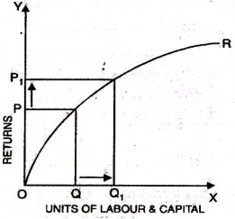
- When proportionate increase in factors of production leads to higher proportionate increase in production refers to increasing return of scale.
- In the below figure, x axis represent increase in labour and capital while Y axis represent increase in output. When labour and capital increases from Q to Q1, output also increases from P to P1 which is higher than the change in factors of production ie labour and capital

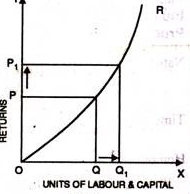
2. Diminishing return of scale
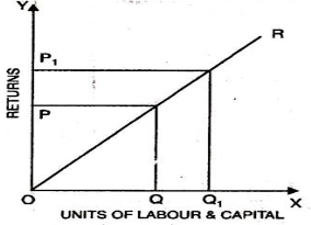
3. Constant return of scale
Q4) Explain cost curve
A4) Short run cost
Short run cost is the cost where the quantity of one input is fixed and the quantity of other input varies. In this case, the land and machinery is fixed where as the other factors such as labour and capital vary with time. Thus expansion is done in hiring more labour and increasing capital.
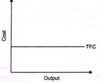
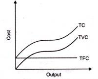
- In the words of Ferguson, “Total fixed cost is the sum of the ‘short run explicit fixed costs and implicit costs incurred by the entrepreneur.”

2. Total variable cost
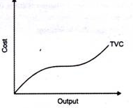
According to Ferguson, “total variable cost is the sum of amounts spent for each of the variable inputs used”
In the above figure, TVC changes with the change in the level of production
3. Total cost

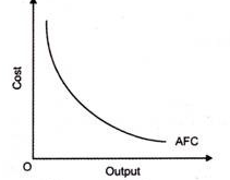
4. Average fixed cost (AFC)–
5. Average variable cost (AVC)
6. Average cost of production (AC)
7. Marginal cost (MC)
 Proportionate change in output
Long run cost
In long run, all the factors of production vary. Long run is period in which all cost change as all the factors of production are variable. To produce at a lower cost in long run, the organization should have the ability to change the factors of production. There is no difference between TC and TVC as there is no fixed cost.
- It refers to the minimum cost at which a given level of output can be produced.
- Definition
According to Leibhafasky, “the long run total cost of production is the least possible cost of producing any given level of output when all inputs are variable.”
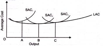
2. Long run average cost (LAC)
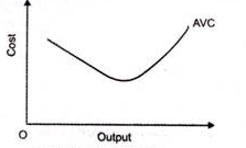
3. Long run marginal cost (LMC)-
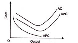
Q5) Explain concept of revenue
A5) The term revenue refers to income obtained by the firm through sale of goods and services at different prices
Definition
In the words of Dooley, ‘the revenue of a firm is its sales, receipts or income’.
Revenue are of 3 types as given below

- Income received by the seller after selling the output is called total revenue
- “Total revenue is the sum of all sales, receipts or income of a firm.” Dooley
- TR = Q x P
Where,
TR – Total Revenue
Q – Quantity of sale (units sold)
P – Price per unit of output
2. Average Revenue
Where, AR – Average Revenue, TR – Total Revenue – Total units sold
3. Marginal revenue
Q6) Explain perfect competition
A6) Perfect competition refers to ‘A market structure in which there are large number of buyers and sellers with a single uniforms price for the product which is determined by the forces of demand & supply.’ The price prevailing in perfect competition market is equilibrium price.
Definition:
It is identified by the existence of the many firm; they all sell an identical products an equivalent way. The supplier is the one who accepts the price."- Vilas
Such market gains when the request for product of every producer is totally elastic. Mrs Joan Robinson.
It is a market condition with an outsized number of sellers and buyers, similar products, free entry of enterprises into the industry is ideal knowledge between buyers and sellers of existing market conditions and free mobility of production factors between alternative uses. Lim Chong-ya
Characteristic of perfect competition:-
1) Large number of seller / seller are price takers: There are many potential sellers selling their commodity in the market. Their number is so large that a single seller cannot influence the market price because each seller sells a small fraction of total market supply. The price of the product is determined on the basis of market demand and market supply of the commodity which is accepted by the firms, thus seller is a price taker and not a price maker.
2) Large number of buyers: There are many buyers in the market. A single buyer cannot influence the price of the commodity because individual demand is a small fraction of total market demand.
3) Homogeneous product: The product sold in the market is homogeneous, i.e. identical in quality and size. There is no difference between the products. The products are perfect substitutes for each other.
4) Free entry and exit: There is freedom for new firms or sellers to enter into the market or industry. There is no legal, economic or any type of restrictions. Similarly, the seller is free to leave the market on industry.
5) Perfect knowledge: The seller and buyers have perfect knowledge about the market such as price, demand and supply. This will prevent the buyer from paying higher price than the market price. Similarly, sellers cannot change a different price than the prevailing market price.
6) Perfect mobility of factors of production: Factors of production are freely mobile from one firm to another or from one place to another. This ensures freedom of entry and exit firms. This also ensure that the factors cost are the same for all firms.
7) No transport cost: It is assumed that there are no transport costs. As a result, there is no possibility of changing a higher price on the behalf of transport costs.
8) Non intervention by the government: It is assumed that government does not interfere in the working of the market economy. Price is determined freely according to demand and supply conditions of the market.
9) Single Price: In Perfect Competition all units of a commodity have uniforms or a single price. It is determined by the forces of demand and supply.
Q7) Explain monopoly
A7) The word monopoly has been derived from the combination of two words i.e., ‘Mono’ and ‘Poly’. Mono refers to a single and poly to control.
Thus, monopoly refers to a market situation in which there is only one seller of a commodity.
In monopoly market, single firm or one seller controls the entire market. The firm has all the market power, so he can set the prices to earn more profit as the consumers do not have any alternative.
Definition
“Pure monopoly is represented by a market situation in which there is a single seller of a product for which there are no substitutes; this single seller is unaffected by and does not affect the prices and outputs of other products sold in the economy.” Bilas
“Monopoly is a market situation in which there is a single seller. There are no close substitutes of the commodity it produces, there are barriers to entry”. –Koutsoyiannis
“A pure monopoly exists when there is only one producer in the market. There are no dire competitions.” –Ferguson
Features
2. No Close Substitutes - There is no close substitutes for the product sold by the monopolist. The cross elasticity of demand between the product of the monopolist and others must be negligible or zero.
3. Difficulty of Entry of New Firms - There are restrictions on the entry of firms into the industry, even when the firm is making abnormal profits. Other sellers are unable to enter the market of the monopoly
4. Profit maximizer: a monopoly maximizes profits. Due to the lack of competition a firm can charge a set price above what would be charged in a competitive market, thereby maximizing its revenue.
5. Price Maker - Under monopoly, monopolist has full control over the supply of the commodity. The price is set by determining the quantity in order to demand the price desired by the firm. Therefore, buyers have to pay the price fixed by the monopolist.
Q8) Explain perfect competition equilibrium
A8) Equilibrium of the firm and the industry in the short and the long runs
Equilibrium refers to when the firm has no inclination to expand or to contract its output. The producer can attain equilibrium under two situations.
The Marginal Revenue-Marginal Cost Approach
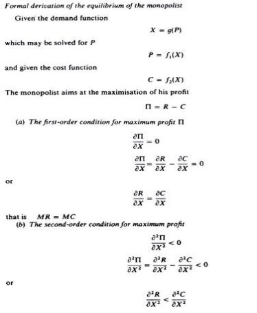
Profit depends on revenue and cost. Thus equilibrium revolves around revenue and cost. According to the MR-MC approach, a producer is said to be in equilibrium when:
- A Firm can maximise the profit when marginal revenue is equal to marginal cost
- MR is the addition to TR from the sale of one more unit
- MC is the addition to TC when an additional unit is produced.
- Thus when MR = MC, TR-TC result in maximum profit.
- If MR exceeds MC, then producer will produce more as it adds to the profit
MC is greater than MR after the MC=MR Output Level
MC= MR is a necessary condition, but its is not enough to ensure equilibrium. This condition happens more than one output level.
To ensure equilibrium, it has to be supplemented by the condition that MR should be less than MC after this level
Producer’s Equilibrium when Price remains Constant
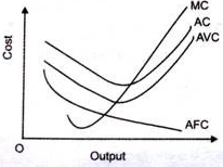
Price remains constant under conditions of perfect competition. Here price is equal to AR. When price is constant, revenue from each additional unit is equal to AR. It means AR curve is same as MR curve. The firm attains equilibrium when two condition are fulfilled , that is firm aims at producing that level of output at which MC is equal to MR and MC is greater than MR after MC = MR output level.
Producer’s Equilibrium when Price is not Constant
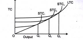
When there is no fixed price, price falls with an increase in output. The producer sells more units at a lower price. In this case MR slopes downwards. The firm aims at producing that level of output at which MC is equal to MR and MC is greater than MR.
Short run and long run supply curves
Supply curve shows the relationship between price and quantity supplied. According to Dorfman, “Supply curve is that curve which indicates various quantities supplied by the firm at different prices”.
Supply curve can be divided into two parts as:
Short run supply curve of a firm
Under Short run , fixed cost remains constant, supply can be changed by changing the only the variable factors. Thus the firm has to bear fixed cost id it is shut down. Thus in short run, goods are supplied at price is either greater or equal to average variable cost. Average revenue is equal to marginal revenue under perfect competition. Hence the firm will produce at the point where marginal revenue and marginal cost are equal.
Prof. Bilas has defined it in simple words, “The Firm’s short period supply curve is that portion of its marginal cost curve that lies-above the minimum point of the average variable cost curve.”
From the above figure we can see that, the firm will not be covering its average variable cost, at price less than OP. At price OP, OM is the supply. MC and MR cut at point A, OM is equilibrium output. If price rise to OP1, the firm will produce OM1 output. This short run supply curve of a firm starts from A upwards i.e., thick line AB.
Long run supply curve
Under long run, the supply curve changes by changing all the factors of production. The firm produces only at minimum average cost in long run. In this case, long run marginal cost, marginal revenue, average revenue and long run average cost are equal. The firm enjoys normal profit.
Optimum production is the point where minimum average cost is equal to marginal cost. Long run supply curve is a portion where marginal cost curve that lies above the minimum point of the average cost curve.

Optimum point is the Point E, as at this point MR=LMCAR minimum LAC. The portion of LMC above point E is called long run supply curve
Q9) Explain monopoly equilibrium
A9) Equilibrium
A. Short run
A monopolist maximizes his short-term profits if the following two conditions are met first, MC equals Mr. Secondly; the slope of MC is larger than that of Mr at the intersection.
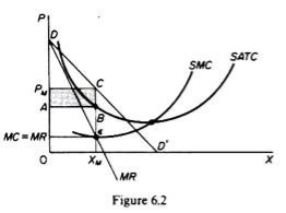
In Figure 6.2, the equilibrium of the monopoly is defined by the point θ at which MC intersects the MR curve from below. Thus, both conditions of equilibrium are met. The price is PM and the quantity is XM. Monopolies realize excess profits equal to shaded areas APM CB. Please note that the price is higher than Mr
In pure competition, the company is the one who receives the price, so it’s only decision is the output decision. The monopolist is faced with two decisions: to set his price and his output. But given the downward trend demand curve, the two decisions are interdependent.
Monopolies set their own prices and sell the amount the market takes on it, or produce an output defined by the intersection of MC and MR and are sold at the corresponding price. An important condition for maximizing the profits of monopolies is the equality of the MC and the MR, provided that the MC cuts the MR from below.

We can now revisit the statement that there is no unique supply curve for the monopolist derived from his MC. Given his MC, the same amount could be offered at different prices depending on the price elasticity of demand. This is graphically shown in Figure 6.3. Quantity X is sold at price P1 if demand is D1, and the same quantity X is sold at price P2 if demand is D2.
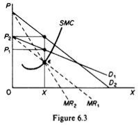
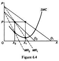
So there is no inherent relationship between price and quantity. Similarly, given the monopolist MC, we can supply various quantities at any one price, depending on the market demand and the corresponding MR curve. Figure 6.4 illustrates this situation. The cost condition is represented by the MC curve. Given the cost of a monopolist, he would supply 0X1 if the market demand is D1, then p at the same price, and only 0X2 if the market demand is D2 B.Long-term equilibrium:
In the long run the monopolist will have time to expand his plants or use his existing plants at every level to maximize his profits. However, if the entry is blocked, the monopolist does not need to reach the optimal scale (that is, the need to build the plant until the minimum point of LAC is reached), neither does the guarantee that he will use his existing plant at the optimum capacity. What is certain is that if he makes a loss in the long run, the monopolist will not stay in business.
He will probably continue to earn paranormal benefits even in the long run, given that entry is banned. But the size of his plant and the degree of utilization of any plant size depends entirely on the market demand. He may reach the optimal scale (the minimum point of Lac), stay on the less optimal scale (the falling part of his LAC), or exceed the optimal scale (expand beyond the minimum LAC), depending on market conditions.
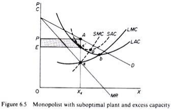
Figure 6.5 shows when the market size does not allow the monopolist to expand to the minimum point of Lac. In this case, not only is his plant not optimal (in the sense that the economy of full size is not depleted), but also the existing plant is not fully utilized. This is because on the left of the minimum point of the LAC, the SRAC touches the LAC at its falling part, and the short-term MC must be equal to the LRMC. This happens in e, but the minimum LAC is b,and the optimal use of the existing plant is a. Since it is utilized at Level E', there is excess capacity. Finally, figure 6.7 shows a case where the market size is large enough for a monopolist to build an optimal plant and be able to use it at full capacity.
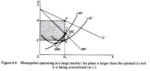
In Figure 6.6, the scale of the market is so large that monopolists have to build plants larger than the optimal ones to maximize output and over-exploit them. This is because to the right of the minimum point of LAC, SRAC and LAC is tangent at the point of positive slope, and SRMC must be equal to LAC. Thus, plants that maximize the profits of monopolies are, firstly, larger than the optimal size, and secondly, they are over-utilized, which leads to higher costs. This is often the case with utility companies operating at the state level.
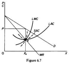
It should be clear that which of the above situations will appear in a particular case will depend on the size of the market (given the technology of monopolists). There is no certainty that monopolies will reach their optimal size in the long run, as is the case with purely competitive markets. In Monopoly, there is no market force similar to those of pure competition that will lead companies to operate at optimal plant size in the long run (and utilize it at its full capacity).
Q10) Explain Explicit and implicit cost, actual and opportunity cost, accounting and economic cost, Social and private costs
A10) Explicit and implicit cost –
Actual and opportunity cost
Accounting and economic cost,
Social and private costs,