Unit – II
Correlation Analysis
Q1) Explain Scattered diagram.
A1)
The more the points plotted are scattered over the chart, the lesser is the degree of correlation between the variables. The more the points plotted are closer to the line, the higher is the degree of correlation. The degree of correlation is denoted by “r”.
a) Perfect positive correlation (r = +1) – All the points plotted on the straight line rising from left to right.
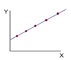
b) Perfect negative correlation (r=-1) – all the points plotted on the straight line falling from left to right.
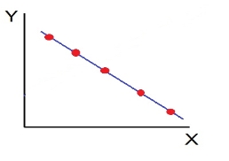
c) High Degree of +Ve Correlation (r= + High): all the points plotted close to the straight line rising from left to right.
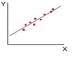
d) High Degree of –Ve Correlation (r= – High) - all the points plotted close to the straight line falling from left to right.
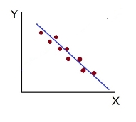
e) Low degree of +Ve Correlation (r= + Low): all the points are highly scattered to the straight line rising from left to right.
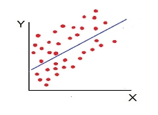
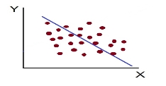
f) Low Degree of –Ve Correlation (r= - Low): all the points are highly scattered to the straight line falling from left to right.
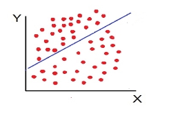
g) No Correlation (r= 0) – all the points are scattered over the graph and do not show any pattern.
Q2) Compute Pearsons coefficient of correlation between advertisement cost and sales as per the data given below:
Advertisement cost | 39 | 65 | 62 | 90 | 82 | 75 | 25 | 98 | 36 | 78 |
sales | 47 | 53 | 58 | 86 | 62 | 68 | 60 | 91 | 51 | 84 |
A2)
X | Y |
|
|
|
| |
39 | 47 | -26 | 676 | -19 | 361 | 494 |
65 | 53 | 0 | 0 | -13 | 169 | 0 |
62 | 58 | -3 | 9 | -8 | 64 | 24 |
90 | 86 | 25 | 625 | 20 | 400 | 500 |
82 | 62 | 17 | 289 | -4 | 16 | -68 |
75 | 68 | 10 | 100 | 2 | 4 | 20 |
25 | 60 | -40 | 1600 | -6 | 36 | 240 |
98 | 91 | 33 | 1089 | 25 | 625 | 825 |
36 | 51 | -29 | 841 | -15 | 225 | 435 |
78 | 84 | 13 | 169 | 18 | 324 | 234 |
650 | 660 |
| 5398 |
| 2224 | 2704 |
|
|
|
|
|
|
|

r = (2704)/√5398 √2224 = (2704)/(73.2*47.15) = 0.78
Thus, Correlation coefficient is positively correlated
Q3) Find Spearman's rank correlation coefficient between X and Y for this set of data:
X | 13 | 20 | 22 | 18 | 19 | 11 | 10 | 15 |
Y | 17 | 19 | 23 | 16 | 20 | 10 | 11 | 18 |
A3)
X | Y | Rank X | Rank Y | d | d2 |
13 | 17 | 3 | 4 | -1 | 1 |
20 | 19 | 7 | 6 | 1 | 1 |
22 | 23 | 8 | 8 | 0 | 0 |
18 | 16 | 5 | 3 | 2 | 2 |
19 | 20 | 6 | 7 | -1 | 1 |
11 | 10 | 2 | 1 | 1 | 1 |
10 | 11 | 1 | 2 | -1 | 1 |
15 | 18 | 4 | 5 | -1 | 1 |
|
|
|
|
| 8 |
R =

 R = 1 – 6*8/8(82 – 1) = 1 – 48 = 0.90
504
Q4) Calculation of equal ranks or tie ranks.
Find Spearman's rank correlation coefficient:
Commerce | 15 | 20 | 28 | 12 | 40 | 60 | 20 | 80 |
Science | 40 | 30 | 50 | 30 | 20 | 10 | 30 | 60 |
A4)
C | S | Rank C | Rank S | d | d2 |
15 | 40 | 2 | 6 | -4 | 16 |
20 | 30 | 3.5 | 4 | -0.5 | 0.25 |
28 | 50 | 5 | 7 | -2 | 4 |
12 | 30 | 1 | 4 | -3 | 9 |
40 | 20 | 6 | 2 | 4 | 16 |
60 | 10 | 7 | 1 | 6 | 36 |
20 | 30 | 3.5 | 4 | -0.5 | 0.25 |
80 | 60 | 8 | 8 | 0 | 0 |
|
|
|
|
| 81.5 |

R = 1 – (6*81.5)/8(82 – 1) = 0.02
Q5) Difference between correlation and regression.
A5)
Correlation | Regression |
‘Correlation’ as the name says it determines the interconnection or a co-relationship between the variables. | ‘Regression’ explains how an independent variable is numerically associated with the dependent variable. |
In Correlation, both the independent and dependent values have no difference. | However, in Regression, both the dependent and independent variable are different. |
The primary objective of Correlation is, to find out a quantitative/numerical value expressing the association between the values. | When it comes to regression, its primary intent is, to reckon the values of a haphazard variable based on the values of the fixed variable. |
Correlation stipulates the degree to which both of the variables can move together. | However, regression specifies the effect of the change in the unit, in the known variable(p) on the evaluated variable (q). |
Correlation helps to constitute the connection between the two variables. | Regression helps in estimating a variable’s value based on another given value. |
Q6) How to find a linear regression equation.
Subject | X | Y |
1 | 43 | 99 |
2 | 21 | 65 |
3 | 25 | 79 |
4 | 42 | 75 |
5 | 57 | 87 |
6 | 59 | 81 |
|
|
|
A6)
Subject | X | Y | Xy | X2 | Y2 |
1 | 43 | 99 | 4257 | 1849 | 9801 |
2 | 21 | 65 | 1365 | 441 | 4225 |
3 | 25 | 79 | 1975 | 625 | 6241 |
4 | 42 | 75 | 3150 | 1764 | 5625 |
5 | 57 | 87 | 4959 | 3249 | 7569 |
6 | 59 | 81 | 4779 | 3481 | 6521 |
Total | 247 | 486 | 20485 | 11409 | 40022 |
To find a and b, use the following equation
Find a:
((486 × 11,409) – ((247 × 20,485)) / 6 (11,409) – 247*247)
484979 / 7445
=65.14
Find b:
(6(20,485) – (247 × 486)) / (6 (11409) – 247*247)
(122,910 – 120,042) / 68,454 – 2472
2,868 / 7,445
= .385225
y’ = a + bx
y’ = 65.14 + .385225x
Q7) Find the two regression equation of X on Y and Y on X from the following data:
X: 10 12 16 11 15 14 20 22
Y: 15 18 23 14 20 17 25 28
A7)

Here N = Number of elements in either series X or series Y = 8
Now we will proceed to compute regression equations using normal equations.
Regression equation of X on Y: X = a + bY
The two normal equations are:

Substituting the values in above normal equations, we get
120 = 8a + 160b ..... (i)
2542 = 160a + 3372b ..... (ii)
Let us solve these equations (i) and (ii) by simultaneous equation method
Multiply equation (i) by 20 we get 2400 = 160a + 3200b
Now rewriting these equations:
2400 = 160a + 3200b
2542 = 160a + 3372b
(-) (-) (-) .
-142 = -172b
Therefore, now we have -142 = -172b, this can re-written as 172b = 142
Now, b = 142/172 = 0.8256 (rounded off)
Substituting the value of b in equation (i), we get
120 = 8a + (160 * 0.8256)
120 = 8a + 132 (rounded off)
8a = 120 - 132
8a = -12
a = -12/8
a = -1.5
Thus, we got the values of a = -1.5 and b = 0.8256
Hence the required regression equation of X on Y:
X = a + bY => X = -1.5 + 0.8256Y
Regression equation of Y on X: Y = a + bX
The two normal equations are:
∑Y = Na + b∑X
∑XY = a∑X + b∑X2
Substituting the values in above normal equations, we get
160 = 8a + 120b ..... (iii)
2542 = 120a + 1926b ..... (iv)
Let us solve these equations (iii) and (iv) by simultaneous equation method
Multiply equation (iii) by 15 we get 2400 = 120a + 1800b
Now rewriting these equations:
2400 = 120a + 1800b
2542 = 120a + 1926b
(-) (-) (-) .
-142 = -126b
Therefore, now we have -142 = -126b, this can re-written as 126b = 142
Now, b = 142/126 = 1.127 (rounded off)
Substituting the value of b in equation (iii), we get
160 = 8a + (120 * 1.127)
160 = 8a + 135.24
8a = 160 - 135.24
8a = 24.76
a = 24.76/8
a = 3.095
Thus, we got the values of a = 3.095 and b = 1.127
Hence the required regression equation of Y on X:
Y = a + bX => Y = 3.095 + 1.127X
Q8) Compute correlation coefficient from the following data
Hours of sleep (X) | Test scores (Y) |
8 | 81 |
8 | 80 |
6 | 75 |
5 | 65 |
7 | 91 |
6 | 80 |
A8)
X | Y |
|
|
|
| |
8 | 81 | 1.3 | 1.8 | 2.3 | 5.4 | 3.1 |
8 | 80 | 1.3 | 1.8 | 1.3 | 1.8 | 1.8 |
6 | 75 | -0.7 | 0.4 | -3.7 | 13.4 | 2.4 |
5 | 65 | -1.7 | 2.8 | -13.7 | 186.8 | 22.8 |
7 | 91 | 0.3 | 0.1 | 12.3 | 152.1 | 4.1 |
6 | 80 | -0.7 | 0.4 | 1.3 | 1.8 | -0.9 |
40 | 472 |
| 7 |
| 361 | 33 |

X = 40/6 =6.7

Y = 472/6 = 78.7

r = (33)/√7 √361 = (33)/(2.64*19) = 0.66
Thus, Correlation coefficient is positively correlated
Q9) Calculate coefficient of correlation between X and Y series using Karl Pearson shortcut method
X | 14 | 12 | 14 | 16 | 16 | 17 | 16 | 15 |
Y | 13 | 11 | 10 | 15 | 15 | 9 | 14 | 17 |
A9)
Let assumed mean for X = 15, assumed mean for Y = 14
X | Y | dx | dx2 | dy | dy2 | dxdy |
14 | 13 | -1.0 | 1.0 | -1.0 | 1.0 | 1.0 |
12 | 11 | -3.0 | 9.0 | -3.0 | 9.0 | 9.0 |
14 | 10 | -1.0 | 1.0 | -4.0 | 16.0 | 4.0 |
16 | 15 | 1.0 | 1.0 | 1.0 | 1.0 | 1.0 |
16 | 15 | 1.0 | 1.0 | 1.0 | 1.0 | 1.0 |
17 | 9 | 2.0 | 4.0 | -5.0 | 25.0 | -10.0 |
16 | 14 | 1 | 1 | 0 | 0 | 0 |
15 | 17 | 0 | 0 | 3 | 9 | 0 |
120 | 104 | 0 | 18 | -8 | 62 | 6 |

 r = 8 *6 – (0)*(-8)
√8*18-(0)2 √8*62 – (-8)2
r = 48/√144*√432 = 0.19
Q10) Calculate coefficient of correlation between X and Y series using Karl pearson shortcut method
X | 1800 | 1900 | 2000 | 2100 | 2200 | 2300 | 2400 | 2500 | 2600 |
F | 5 | 5 | 6 | 9 | 7 | 8 | 6 | 8 | 9 |
A10)
Assumed mean of X and Y is 2200, 6
X | Y | dx | dx (i=100) | dx2 | dy | dy2 | dxdy |
1800 | 5 | -400 | -4 | 16 | -1.0 | 1.0 | 4.0 |
1900 | 5 | -300 | -3 | 9 | -1.0 | 1.0 | 3.0 |
2000 | 6 | -200 | -2 | 4 | 0.0 | 0.0 | 0.0 |
2100 | 9 | -100 | -1 | 1 | 3.0 | 9.0 | -3.0 |
2200 | 7 | 0 | 0 | 0 | 1.0 | 1.0 | 0.0 |
2300 | 8 | 100 | 1 | 1 | 2.0 | 4.0 | 2.0 |
2400 | 6 | 200 | 2 | 4 | 0 | 0 | 0.0 |
2500 | 8 | 300 | 3 | 9 | 2 | 4 | 6.0 |
2600 | 9 | 400 | 4 | 16 | 3 | 9 | 12.0 |
|
|
|
|
|
|
|
|
|
|
| 0 | 60 | 9 | 29 | 24 |
Note – we can also proceed dividing x/100
 r = (9)(24) – (0)(9)
√9*60-(0)2 √9*29– (9)2
r = 0.69


